Tutorial

There are two main concepts to understand in SwarmPAL, data and processes. Data live within a xarray DataTree, and processes behave like functions (and are of type PalProcess). Processes act on data to transform them by adding derived parameters into the data object.

We logically separate a workflow into two steps:

• fetching data: data are downloaded from VirES or any HAPI server

• applying processes: apply a “PalProcess” to your data to perform a given analysis routine

Fetching data

Data are pulled in over the web and organised as a DataTree, which is done using create_paldata and PalDataItem:

from swarmpal.io import create_paldata, PalDataItem

data = create_paldata(
    PalDataItem.from_vires(
        server_url="https://vires.services/ows",
        collection="SW_OPER_MAGA_LR_1B",
        measurements=["B_NEC"],
        start_time="2020-01-01T00:00:00",
        end_time="2020-01-01T03:00:00",
    ),
    PalDataItem.from_vires(
        server_url="https://vires.services/ows",
        collection="SW_OPER_MAGC_LR_1B",
        measurements=["B_NEC"],
        start_time="2020-01-01T00:00:00",
        end_time="2020-01-01T03:00:00",
    ),
)
print(data)

<xarray.DataTree 'paldata'>
Group: /
├── Group: /SW_OPER_MAGA_LR_1B
│       Dimensions:     (Timestamp: 10800, NEC: 3)
│       Coordinates:
│         * Timestamp   (Timestamp) datetime64[s] 86kB 2020-01-01 ... 2020-01-01T02:5...
│         * NEC         (NEC) <U1 12B 'N' 'E' 'C'
│       Data variables:
│           Spacecraft  (Timestamp) object 86kB 'A' 'A' 'A' 'A' 'A' ... 'A' 'A' 'A' 'A'
│           B_NEC       (Timestamp, NEC) float64 259kB 3.137e+03 387.8 ... 4.077e+04
│           Radius      (Timestamp) float64 86kB 6.803e+06 6.803e+06 ... 6.806e+06
│           Longitude   (Timestamp) float64 86kB 103.0 103.1 103.1 ... 49.91 49.91 49.91
│           Latitude    (Timestamp) float64 86kB 76.7 76.76 76.82 ... 51.04 51.11 51.17
│       Attributes:
│           Sources:         ['SW_OPER_MAGA_LR_1B_20200101T000000_20200101T235959_070...
│           MagneticModels:  []
│           AppliedFilters:  []
│           PAL_meta:        {"analysis_window": ["2020-01-01T00:00:00", "2020-01-01T...
└── Group: /SW_OPER_MAGC_LR_1B
        Dimensions:     (Timestamp: 10800, NEC: 3)
        Coordinates:
          * Timestamp   (Timestamp) datetime64[s] 86kB 2020-01-01 ... 2020-01-01T02:5...
          * NEC         (NEC) <U1 12B 'N' 'E' 'C'
        Data variables:
            Spacecraft  (Timestamp) object 86kB 'C' 'C' 'C' 'C' 'C' ... 'C' 'C' 'C' 'C'
            B_NEC       (Timestamp, NEC) float64 259kB 2.996e+03 325.2 ... 4.117e+04
            Radius      (Timestamp) float64 86kB 6.803e+06 6.803e+06 ... 6.805e+06
            Longitude   (Timestamp) float64 86kB 104.9 104.9 105.0 ... 51.28 51.29 51.29
            Latitude    (Timestamp) float64 86kB 77.21 77.27 77.33 ... 51.57 51.63 51.69
        Attributes:
            Sources:         ['SW_OPER_MAGC_LR_1B_20200101T000000_20200101T235959_070...
            MagneticModels:  []
            AppliedFilters:  []
            PAL_meta:        {"analysis_window": ["2020-01-01T00:00:00", "2020-01-01T...

The DataTree is the top-level data structure within Xarray and allows organising any number of datasets in a hierarchical way (like a directory tree in a file system). In this example, the data variable is an instance of DataTree containing Swarm data grouped by collections (SW_OPER_MAGA_LR_1B and SW_OPER_MAGC_LR_1B). Each group independently contains dimensions, coordinates, data variables, and attributes that describe the data.

When we use PalDataItem.from_vires, data are fetched from the VirES service (using the viresclient package underneath). Similarly, we can use PalDataItem.from_hapi to fetch data from any HAPI server (which uses hapiclient underneath).

create_paldata and PalDataItem have a few features for flexible use:

• Pass multiple items to create_paldata to assemble a complex datatree. Pass them as keyword arguments (e.g. HAPI_SW_OPER_MAGA_LR_1B=... below) if you want to manually change the name in the datatree, otherwise they will default to the collection/dataset name.

• Use .from_vires() and .from_hapi() to fetch data from different services. Note that the argument names and usage are a bit different (though equivalent) in each case. These follow the nomenclature used in viresclient and hapiclient respectively.

For example:

data = create_paldata(
    PalDataItem.from_vires(
        server_url="https://vires.services/ows",
        collection="SW_OPER_MAGA_LR_1B",
        measurements=["B_NEC"],
        start_time="2020-01-01T00:00:00",
        end_time="2020-01-01T03:00:00",
    ),
    HAPI_SW_OPER_MAGA_LR_1B=PalDataItem.from_hapi(
        server="https://vires.services/hapi",
        dataset="SW_OPER_MAGA_LR_1B",
        parameters="Latitude,Longitude,Radius,B_NEC",
        start="2020-01-01T00:00:00",
        stop="2020-01-01T03:00:00",
    ),
)

While you can learn more about using datatrees on the xarray documentation, this should not be necessary for basic usage of SwarmPAL. If you are familiar with xarray, you can access a dataset by browsing the datatree like a dictionary, then using either the .ds accessor to get an immutable view of the dataset, or .to_dataset() to extract a mutable copy.

data["SW_OPER_MAGA_LR_1B"].ds

<xarray.DatasetView> Size: 691kB
Dimensions:     (Timestamp: 10800, NEC: 3)
Coordinates:
  * Timestamp   (Timestamp) datetime64[s] 86kB 2020-01-01 ... 2020-01-01T02:5...
  * NEC         (NEC) <U1 12B 'N' 'E' 'C'
Data variables:
    Spacecraft  (Timestamp) object 86kB 'A' 'A' 'A' 'A' 'A' ... 'A' 'A' 'A' 'A'
    B_NEC       (Timestamp, NEC) float64 259kB 3.137e+03 387.8 ... 4.077e+04
    Radius      (Timestamp) float64 86kB 6.803e+06 6.803e+06 ... 6.806e+06
    Longitude   (Timestamp) float64 86kB 103.0 103.1 103.1 ... 49.91 49.91 49.91
    Latitude    (Timestamp) float64 86kB 76.7 76.76 76.82 ... 51.04 51.11 51.17
Attributes:
    Sources:         ['SW_OPER_MAGA_LR_1B_20200101T000000_20200101T235959_070...
    MagneticModels:  []
    AppliedFilters:  []
    PAL_meta:        {"analysis_window": ["2020-01-01T00:00:00", "2020-01-01T...

xarray.DatasetView

• Dimensions:
  • Timestamp: 10800
  • NEC: 3
• Coordinates: (2)
  • Timestamp
    (Timestamp)
    datetime64[s]
    2020-01-01 ... 2020-01-01T02:59:59

    description :

    Time stamp

    array(['2020-01-01T00:00:00', '2020-01-01T00:00:01', '2020-01-01T00:00:02',
           ..., '2020-01-01T02:59:57', '2020-01-01T02:59:58',
           '2020-01-01T02:59:59'], shape=(10800,), dtype='datetime64[s]')

  • NEC
    (NEC)
    <U1
    'N' 'E' 'C'

    units :

    description :

    NEC frame - North, East, Centre (down)

    array(['N', 'E', 'C'], dtype='<U1')

• Data variables: (5)
  • Spacecraft
    (Timestamp)
    object
    'A' 'A' 'A' 'A' ... 'A' 'A' 'A' 'A'

    units :

    -

    description :

    Spacecraft identifier (values: 'A', 'B', 'C' or '-' if not available).

    array(['A', 'A', 'A', ..., 'A', 'A', 'A'], shape=(10800,), dtype=object)

  • B_NEC
    (Timestamp, NEC)
    float64
    3.137e+03 387.8 ... 4.077e+04

    units :

    nT

    description :

    Magnetic field vector, NEC frame

    array([[ 3136.7844,   387.8261, 48680.0214],
           [ 3116.5456,   388.2548, 48674.0282],
           [ 3096.6464,   388.629 , 48667.9733],
           ...,
           [15561.0284,  2513.6317, 40711.6148],
           [15531.2407,  2516.2474, 40739.6992],
           [15501.4667,  2518.8121, 40767.7089]], shape=(10800, 3))

  • Radius
    (Timestamp)
    float64
    6.803e+06 6.803e+06 ... 6.806e+06

    units :

    m

    description :

    Position in ITRF - Radius

    array([6802939.9 , 6802936.35, 6802932.82, ..., 6805541.56, 6805532.03,
           6805522.51], shape=(10800,))

  • Longitude
    (Timestamp)
    float64
    103.0 103.1 103.1 ... 49.91 49.91

    units :

    deg

    description :

    Position in ITRF - Longitude

    array([103.0425829, 103.0947424, 103.1474322, ...,  49.9064435,
            49.909776 ,  49.9131295], shape=(10800,))

  • Latitude
    (Timestamp)
    float64
    76.7 76.76 76.82 ... 51.11 51.17

    units :

    deg

    description :

    Position in ITRF - Latitude

    array([76.6969508, 76.7600937, 76.8232241, ..., 51.0436972, 51.1079599,
           51.1722222], shape=(10800,))

• Attributes: (4)

  Sources :

  ['SW_OPER_MAGA_LR_1B_20200101T000000_20200101T235959_0701_MDR_MAG_LR']

  MagneticModels :

  []

  AppliedFilters :

  []

  PAL_meta :

  {"analysis_window": ["2020-01-01T00:00:00", "2020-01-01T03:00:00"], "magnetic_models": {}, "config": {"pad_times": [], "collection": "SW_OPER_MAGA_LR_1B", "measurements": ["B_NEC"], "start_time": "2020-01-01T00:00:00", "end_time": "2020-01-01T03:00:00", "server_url": "https://vires.services/ows", "models": [], "auxiliaries": [], "sampling_step": null, "filters": [], "options": {}, "provider": "vires"}}

Using the VirES API, there are additional things that can be requested outwith the original dataset (models and auxiliaries). See the viresclient documentation for details, or Swarm Notebooks for more examples. The extra options below specifies an extendable dictionary of special options which are passed to viresclient. In this case we specify asynchronous=False to process the request synchronously (faster, but will fail for longer requests), and disable the progress bars with show_progress=False.

data = create_paldata(
    PalDataItem.from_vires(
        server_url="https://vires.services/ows",
        collection="SW_OPER_MAGA_LR_1B",
        measurements=["B_NEC"],
        models=["IGRF"],
        auxiliaries=["QDLat", "MLT"],
        start_time="2020-01-01T00:00:00",
        end_time="2020-01-01T03:00:00",
        options=dict(asynchronous=False, show_progress=False),
    )
)
print(data)

<xarray.DataTree 'paldata'>
Group: /
└── Group: /SW_OPER_MAGA_LR_1B
        Dimensions:     (Timestamp: 10800, NEC: 3)
        Coordinates:
          * Timestamp   (Timestamp) datetime64[s] 86kB 2020-01-01 ... 2020-01-01T02:5...
          * NEC         (NEC) <U1 12B 'N' 'E' 'C'
        Data variables:
            Spacecraft  (Timestamp) object 86kB 'A' 'A' 'A' 'A' 'A' ... 'A' 'A' 'A' 'A'
            Radius      (Timestamp) float64 86kB 6.803e+06 6.803e+06 ... 6.806e+06
            QDLat       (Timestamp) float64 86kB 71.96 72.02 72.08 ... 47.41 47.47 47.54
            B_NEC_IGRF  (Timestamp, NEC) float64 259kB 3.14e+03 405.3 ... 4.076e+04
            Latitude    (Timestamp) float64 86kB 76.7 76.76 76.82 ... 51.04 51.11 51.17
            B_NEC       (Timestamp, NEC) float64 259kB 3.137e+03 387.8 ... 4.077e+04
            MLT         (Timestamp) float64 86kB 6.569 6.571 6.574 ... 6.172 6.173 6.174
            Longitude   (Timestamp) float64 86kB 103.0 103.1 103.1 ... 49.91 49.91 49.91
        Attributes:
            Sources:         ['SW_OPER_AUX_IGR_2__19000101T000000_20291231T235959_010...
            MagneticModels:  ['IGRF = IGRF(max_degree=13,min_degree=1)']
            AppliedFilters:  []
            PAL_meta:        {"analysis_window": ["2020-01-01T00:00:00", "2020-01-01T...

Applying Processes

A process is a special object type you can import from different toolboxes in SwarmPAL.

First we import the relevant toolbox and create a process from the .processes submodule:

from swarmpal.toolboxes import fac

process = fac.processes.FAC_single_sat()

Each process has a .set_config() method which configures the behaviour of the process:

help(process.set_config)

Help on method set_config in module swarmpal.toolboxes.fac.processes:

set_config(dataset: 'str' = 'SW_OPER_MAGA_LR_1B', model_varname: 'str' = 'B_NEC_CHAOS', measurement_varname: 'str' = 'B_NEC', inclination_limit: 'float' = 30, time_jump_limit: 'int' = 1, include_auxiliaries: 'bool' = True, output_dataset: 'str' = 'PAL_FAC_single_sat') -> 'None' method of swarmpal.toolboxes.fac.processes.FAC_single_sat instance
    Configures the process
    
    Parameters
    ----------
    dataset : str, optional
        Dataset to use, by default "SW_OPER_MAGA_LR_1B"
    model_varname : str, optional
        Name of the magnetic model predictions, by default "B_NEC_Model"
    measurement_varname : str, optional
        Name of the measurements, by default "B_NEC"
    inclination_limit : float, optional
        Limit of inclination for FAC validity (in degrees), by default 30
    time_jump_limit : int, optional
        Maximum allowable time step in data for FAC validity (in seconds), by default 1
    include_auxiliaries : bool, optional
        Whether to include e.g. Latitude, Longitude, Flags, etc, by default True
    output_dataset : str
        Sets the name of the dataset in the data tree that TFA processes will write results to, by default "PAL_FAC_singlesat"

process.set_config(
    dataset="SW_OPER_MAGA_LR_1B",
    model_varname="B_NEC_IGRF",
    measurement_varname="B_NEC",
)

Processes are callable, which means they can be used like functions. They act on datatrees to alter them. We can use this process on the the data we built above.

data = process(data)
print(data)

<xarray.DataTree 'paldata'>
Group: /
│   Attributes:
│       PAL_meta:  {"output_datasets": ["PAL_FAC_single_sat"]}
├── Group: /SW_OPER_MAGA_LR_1B
│       Dimensions:     (Timestamp: 10800, NEC: 3)
│       Coordinates:
│         * Timestamp   (Timestamp) datetime64[s] 86kB 2020-01-01 ... 2020-01-01T02:5...
│         * NEC         (NEC) <U1 12B 'N' 'E' 'C'
│       Data variables:
│           Spacecraft  (Timestamp) object 86kB 'A' 'A' 'A' 'A' 'A' ... 'A' 'A' 'A' 'A'
│           Radius      (Timestamp) float64 86kB 6.803e+06 6.803e+06 ... 6.806e+06
│           QDLat       (Timestamp) float64 86kB 71.96 72.02 72.08 ... 47.41 47.47 47.54
│           B_NEC_IGRF  (Timestamp, NEC) float64 259kB 3.14e+03 405.3 ... 4.076e+04
│           Latitude    (Timestamp) float64 86kB 76.7 76.76 76.82 ... 51.04 51.11 51.17
│           B_NEC       (Timestamp, NEC) float64 259kB 3.137e+03 387.8 ... 4.077e+04
│           MLT         (Timestamp) float64 86kB 6.569 6.571 6.574 ... 6.172 6.173 6.174
│           Longitude   (Timestamp) float64 86kB 103.0 103.1 103.1 ... 49.91 49.91 49.91
│       Attributes:
│           Sources:         ['SW_OPER_AUX_IGR_2__19000101T000000_20291231T235959_010...
│           MagneticModels:  ['IGRF = IGRF(max_degree=13,min_degree=1)']
│           AppliedFilters:  []
│           PAL_meta:        {"analysis_window": ["2020-01-01T00:00:00", "2020-01-01T...
└── Group: /PAL_FAC_single_sat
        Dimensions:    (Timestamp: 10799)
        Coordinates:
          * Timestamp  (Timestamp) datetime64[ns] 86kB 2020-01-01T00:00:00.500000 ......
        Data variables:
            FAC        (Timestamp) float64 86kB -0.04896 -0.06002 ... -0.007683
            IRC        (Timestamp) float64 86kB 0.04886 0.0599 ... 0.002769 0.007168
            Radius     (Timestamp) float64 86kB nan nan nan nan nan ... nan nan nan nan
            Longitude  (Timestamp) float64 86kB nan nan nan nan nan ... nan nan nan nan
            Latitude   (Timestamp) float64 86kB nan nan nan nan nan ... nan nan nan nan
        Attributes:
            Sources:   ['SW_OPER_AUX_IGR_2__19000101T000000_20291231T235959_0104', 'S...
            PAL_meta:  {"FAC_single_sat": {"output_dataset": "PAL_FAC_single_sat", "d...

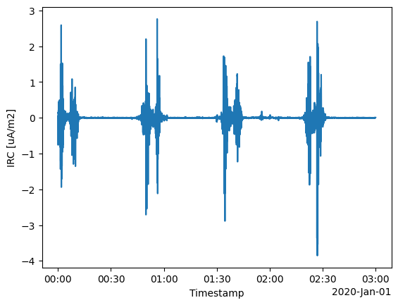
The data has been modified, in this case adding a new group called PAL_FAC_single_sat. We can inspect it using the usual xarray/matplotlib tooling, for example:

data["PAL_FAC_single_sat"]["IRC"].plot.line(x="Timestamp")

[<matplotlib.lines.Line2D at 0x788f4aa44390>]

Saving/loading data

Since data is just a normal datatree, we can use the usual xarray tools to write and read files. Some situations this might be useful in are:

• Saving preprocessed (i.e. interim) data, then later reloading it for further processing. One might download a whole series of data, then in a second, more iterative workflow, analyse it (without having to wait again for the download)

• Saving the output of a process to use in other tools

• Saving the output of a process to later reload just for visualisation

from os import remove
from xarray import open_datatree

# Save the file as NetCDF
data.to_netcdf("testdata.nc")
# Load the data as a new datatree
reloaded_data = open_datatree("testdata.nc")
# Remove that file we just made
remove("testdata.nc")
print(reloaded_data)

<xarray.DataTree>
Group: /
│   Attributes:
│       PAL_meta:  {"output_datasets": ["PAL_FAC_single_sat"]}
├── Group: /SW_OPER_MAGA_LR_1B
│       Dimensions:     (Timestamp: 10800, NEC: 3)
│       Coordinates:
│         * Timestamp   (Timestamp) datetime64[ns] 86kB 2020-01-01 ... 2020-01-01T02:...
│         * NEC         (NEC) <U1 12B 'N' 'E' 'C'
│       Data variables:
│           Spacecraft  (Timestamp) <U1 43kB ...
│           Radius      (Timestamp) float64 86kB ...
│           QDLat       (Timestamp) float64 86kB ...
│           B_NEC_IGRF  (Timestamp, NEC) float64 259kB ...
│           Latitude    (Timestamp) float64 86kB ...
│           B_NEC       (Timestamp, NEC) float64 259kB ...
│           MLT         (Timestamp) float64 86kB ...
│           Longitude   (Timestamp) float64 86kB ...
│       Attributes:
│           Sources:         ['SW_OPER_AUX_IGR_2__19000101T000000_20291231T235959_010...
│           MagneticModels:  IGRF = IGRF(max_degree=13,min_degree=1)
│           AppliedFilters:  []
│           PAL_meta:        {"analysis_window": ["2020-01-01T00:00:00", "2020-01-01T...
└── Group: /PAL_FAC_single_sat
        Dimensions:    (Timestamp: 10799)
        Coordinates:
          * Timestamp  (Timestamp) datetime64[ns] 86kB 2020-01-01T00:00:00.500000 ......
        Data variables:
            FAC        (Timestamp) float64 86kB ...
            IRC        (Timestamp) float64 86kB ...
            Radius     (Timestamp) float64 86kB ...
            Longitude  (Timestamp) float64 86kB ...
            Latitude   (Timestamp) float64 86kB ...
        Attributes:
            Sources:   ['SW_OPER_AUX_IGR_2__19000101T000000_20291231T235959_0104', 'S...
            PAL_meta:  {"FAC_single_sat": {"output_dataset": "PAL_FAC_single_sat", "d...

The .swarmpal accessor

Whenever you import swarmpal, this registers an accessor to datatrees, with extra tools available under <datatree>.swarmpal.<...>. One way in which this is used is to read metadata (stored within the datatree). Here we see that the Preprocess process from the FAC toolbox has saved the configuration which was used:

reloaded_data.swarmpal.pal_meta

{'.': {'output_datasets': ['PAL_FAC_single_sat']},
 'SW_OPER_MAGA_LR_1B': {'analysis_window': ['2020-01-01T00:00:00',
   '2020-01-01T03:00:00'],
  'magnetic_models': {'IGRF': 'IGRF(max_degree=13,min_degree=1)'},
  'config': {'pad_times': [],
   'collection': 'SW_OPER_MAGA_LR_1B',
   'measurements': ['B_NEC'],
   'start_time': '2020-01-01T00:00:00',
   'end_time': '2020-01-01T03:00:00',
   'server_url': 'https://vires.services/ows',
   'models': ['IGRF'],
   'auxiliaries': ['QDLat', 'MLT'],
   'sampling_step': None,
   'filters': [],
   'options': {'asynchronous': False, 'show_progress': False},
   'provider': 'vires'}},
 'PAL_FAC_single_sat': {'FAC_single_sat': {'output_dataset': 'PAL_FAC_single_sat',
   'dataset': 'SW_OPER_MAGA_LR_1B',
   'model_varname': 'B_NEC_IGRF',
   'measurement_varname': 'B_NEC',
   'inclination_limit': 30,
   'time_jump_limit': 1,
   'include_auxiliaries': True}}}

Since this is stored within the data itself, this is preserved over round trips through files so that a following process can see this information, even in a different session.