Analysis of Swarm Electric Field data

In this example we will use the SW_EXPT_EFIx_TCT02 dataset which includes electric field measurements from the VxB product, in two directions, “horizontal” or “vertical”, both in the instrument XYZ cartesian coordinate frame.

For more information about the data and other ways to access it, see:

• Data handbook

• viresclient documentation

• EFIxTCT demo notebook

import datetime as dt

from swarmpal.io import create_paldata, PalDataItem
from swarmpal.toolboxes import tfa

Fetching data

data_params = dict(
    collection="SW_EXPT_EFIA_TCT02",
    measurements=["Ehx", "Ehy", "Ehz", "Quality_flags"],
    auxiliaries=["QDLat", "MLT"],
    start_time=dt.datetime(2015, 3, 14, 12, 5, 0),
    end_time=dt.datetime(2015, 3, 14, 12, 30, 0),
    pad_times=(dt.timedelta(hours=3), dt.timedelta(hours=3)),
    server_url="https://vires.services/ows",
    options=dict(asynchronous=False, show_progress=False),
)
data = create_paldata(PalDataItem.from_vires(**data_params));

Processing

While the data above contains separate variables for each vector component (“Ehx”, “Ehy”, “Ehz”), the TFA toolbox can interpret the variable “Eh_XYZ” as the combination of these.

Note that this dataset is at 2Hz so we must specify sampling_rate=2.

p1 = tfa.processes.Preprocess()
p1.set_config(
    dataset="SW_EXPT_EFIA_TCT02",
    active_variable="Eh_XYZ",
    active_component=2,
    sampling_rate=2,
)
p2 = tfa.processes.Clean()
p2.set_config(
    window_size=300,
    method="iqr",
    multiplier=1,
)
p3 = tfa.processes.Filter()
p3.set_config(
    cutoff_frequency=20 / 1000,
)
p4 = tfa.processes.Wavelet()
p4.set_config(
    min_frequency=20 / 1000,
    max_frequency=200 / 1000,
    dj=0.1,
)
p1(data)
p2(data)
p3(data)
p4(data);

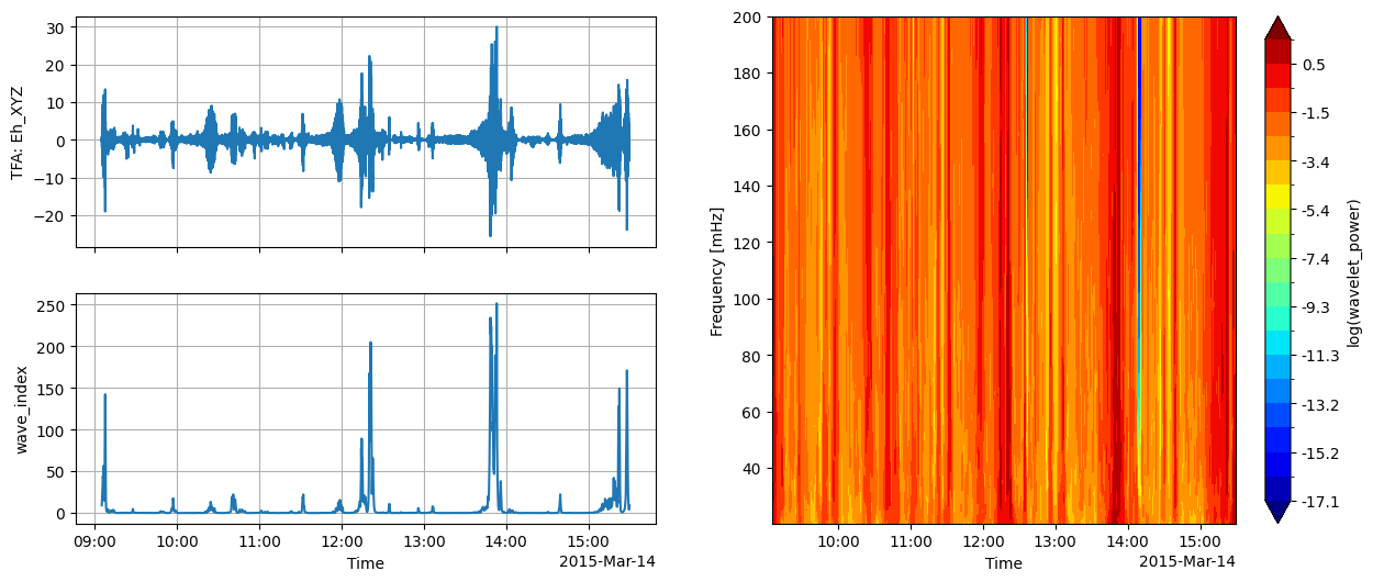
Plotting

tfa.plotting.quicklook(data);