Analysis of Swarm MAG LR data (1Hz)#
For more information about the data and other ways to access it, see:
import datetime as dt
import matplotlib.pyplot as plt

from swarmpal.io import create_paldata, PalDataItem
from swarmpal.toolboxes import tfa
Fetching data#
As in the introduction example, we will fetch the MAG LR data.
data = create_paldata(
    PalDataItem.from_vires(
        collection="SW_OPER_MAGA_LR_1B",
        measurements=["B_NEC"],
        models=["Model=CHAOS"],
        auxiliaries=["QDLat", "MLT"],
        start_time=dt.datetime(2015, 3, 14),
        end_time=dt.datetime(2015, 3, 14, 3, 59, 59),
        pad_times=(dt.timedelta(hours=3), dt.timedelta(hours=3)),
        server_url="https://vires.services/ows",
        options=dict(asynchronous=False, show_progress=False),
    )
)
print(data)
<xarray.DataTree 'paldata'>
Group: /
└── Group: /SW_OPER_MAGA_LR_1B
        Dimensions:      (Timestamp: 35999, NEC: 3)
        Coordinates:
          * Timestamp    (Timestamp) datetime64[s] 288kB 2015-03-13T21:00:00 ... 2015...
          * NEC          (NEC) <U1 12B 'N' 'E' 'C'
        Data variables:
            Spacecraft   (Timestamp) object 288kB 'A' 'A' 'A' 'A' ... 'A' 'A' 'A' 'A'
            Radius       (Timestamp) float64 288kB 6.835e+06 6.835e+06 ... 6.83e+06
            QDLat        (Timestamp) float64 288kB -9.028 -8.964 -8.899 ... 27.18 27.11
            MLT          (Timestamp) float64 288kB 19.82 19.82 19.82 ... 7.813 7.813
            Longitude    (Timestamp) float64 288kB -15.47 -15.47 -15.47 ... 12.1 12.1
            B_NEC_Model  (Timestamp, NEC) float64 864kB 2.175e+04 ... 2.572e+04
            Latitude     (Timestamp) float64 288kB 1.825 1.889 1.953 ... 34.1 34.03
            B_NEC        (Timestamp, NEC) float64 864kB 2.175e+04 ... 2.572e+04
        Attributes:
            Sources:         ['CHAOS-8.1_static.shc', 'SW_OPER_MAGA_LR_1B_20150313T00...
            MagneticModels:  ["Model = 'CHAOS-Core'(max_degree=20,min_degree=1) + 'CH...
            AppliedFilters:  []
            PAL_meta:        {"analysis_window": ["2015-03-14T00:00:00", "2015-03-14T...
Processing#
This time we will use the convert_to_mfa option to rotate the B_NEC vector to the mean-field aligned (MFA) frame. When the MFA frame is used, the active_component must be set to one of (0, 1, 2): 0 is the poloidal component, 1 the toroidal and 2 the compressional. Similarly for B_NEC, the numbers correspond to the North (0), East (1) or Center (2) components.
p1 = tfa.processes.Preprocess()
p1.set_config(
    dataset="SW_OPER_MAGA_LR_1B",
    active_variable="B_MFA",
    active_component=2,
    sampling_rate=1,
    remove_model=True,
    convert_to_mfa=True,
)
p1(data);
Even though B_MFA isn’t available in the original data, this variable becomes available when we select convert_to_mfa=True. For more information on the other options, refer to the documentation:
help(tfa.processes.Preprocess.set_config)
Help on function set_config in module swarmpal.toolboxes.tfa.processes:

set_config(self, dataset: 'str' = '', timevar: 'str' = 'Timestamp', active_variable: 'str' = '', active_component: 'int | None' = None, sampling_rate: 'float' = 1, remove_model: 'bool' = False, model: 'str' = '', convert_to_mfa: 'bool' = False, use_magnitude: 'bool' = False, clean_by_flags: 'bool' = False, flagclean_varname: 'str' = '', flagclean_flagname: 'str' = '', flagclean_maxval: 'int | None' = None, output_dataset: 'str' = 'PAL_TFA') -> 'None'
    Set the process configuration

    Parameters
    ----------
    dataset : str
        Selects this dataset from the datatree
    timevar : str
        Identifies the name of the time variable, usually "Timestamp" or "Time"
    active_variable : str
        Selects the variable to use from within the dataset
    active_component : int, optional
        Selects the component to use (if active_variable is a vector)
    sampling_rate : float, optional
        Identify the sampling rate of the data input (in Hz), by default 1
    remove_model : bool, optional
        Remove a magnetic model prediction or not, by default False
    model : str, optional
        The name of the model
    convert_to_mfa : bool, optional
        Rotate B to mean-field aligned (MFA) coordinates, by default False
    use_magnitude : bool, optional
        Use the magnitude of a vector instead, by default False
    clean_by_flags : bool, optional
        Whether to apply additional flag cleaning or not, by default False
    flagclean_varname : str, optional
        Name of the variable to clean
    flagclean_flagname : str, optional
        Name of the flag to use to clean by
    flagclean_maxval : int, optional
        Maximum allowable flag value
    output_dataset : str
        Sets the name of the dataset in the data tree that TFA processes will write results to, by default "PAL_TFA"

    Notes
    -----
    Some special ``active_variable`` names exist which are added to the dataset on-the-fly:

    * "B_NEC_res_Model"
        where a model prediction must be available in the data, like ``"B_NEC_<Model>"``, and ``remove_model`` has been set. The name of the model can be set with, for example, ``model="CHAOS"``.
    * "B_MFA"
        when ``convert_to_mfa`` has been set.
    * "Eh_XYZ" and "Ev_XYZ"
        when using the TCT datasets, with vectors defined in ``("Ehx", "Ehy", "Ehz")`` and ``("Evx", "Evy", "Evz")`` respectively.
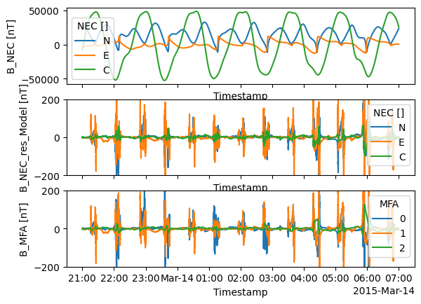
We can inspect the data directly to get an idea about what has happened using Preprocess.
In the figure below, the input B_NEC (first row) and B_NEC_Model have been taken to produce B_NEC_res_Model (second row), and then that has been rotated to the MFA frame (third row). Component “2” is identified from B_MFA and used as the TFA variable (active_component=2 in the above config).
fig, axes = plt.subplots(3, 1, sharex=True)
data["SW_OPER_MAGA_LR_1B"]["B_NEC"].plot.line(x="Timestamp", ax=axes[0])
data["PAL_TFA"]["B_NEC_res_Model"].plot.line(x="Timestamp", ax=axes[1])
data["PAL_TFA"]["B_MFA"].plot.line(x="Timestamp", ax=axes[2])
axes[1].set_ylim(-200, 200)
axes[2].set_ylim(-200, 200);
Let’s prepare the other processes…
p2 = tfa.processes.Clean()
p2.set_config(
window_size=300,
method="iqr",
multiplier=1,
)
p3 = tfa.processes.Filter()
p3.set_config(
cutoff_frequency=20 / 1000,
)
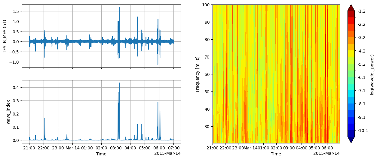
p4 = tfa.processes.Wavelet()
p4.set_config(
min_frequency=20 / 1000,
max_frequency=100 / 1000,
dj=0.1,
)
In practice, you might want to prepare and apply each process in turn to make sure things work right. Here however, we will just apply them all together. Make sure you apply them in the right order!
p2(data)
p3(data)
p4(data);
Plotting#
tfa.plotting.quicklook(data);