TFA and the Wavelet Transform

Here we delve a little into the background of the TFA toolbox.

First we will fetch some data to setup the framework of a typical TFA application, but then we will replace the data with dummy data to demonstrate what the TFA toolbox does.

import datetime as dt
import matplotlib.pyplot as plt
import numpy as np

from swarmpal.io import create_paldata, PalDataItem
from swarmpal.toolboxes import tfa

Get some data and apply the preprocessing.

data = create_paldata(
    PalDataItem.from_vires(
        collection="SW_OPER_MAGA_LR_1B",
        measurements=["F"],
        start_time=dt.datetime(2015, 3, 18),
        end_time=dt.datetime(2015, 3, 18, 0, 15, 0),
        server_url="https://vires.services/ows",
        options=dict(asynchronous=False, show_progress=False),
    )
)

p1 = tfa.processes.Preprocess()
p1.set_config(
    dataset="SW_OPER_MAGA_LR_1B",
    active_variable="F",
    sampling_rate=1,
)
p1(data);

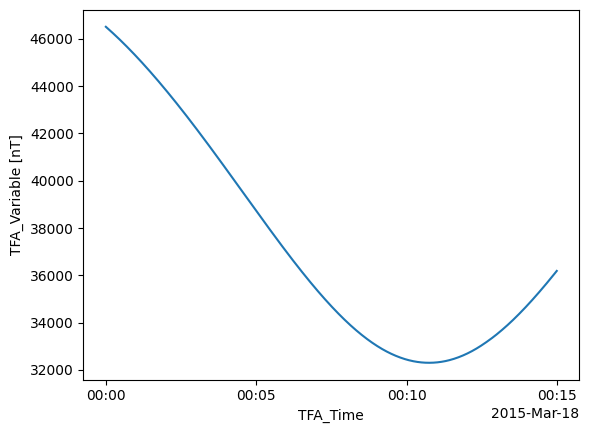
The TFA_Variable has been set with the content of F (the scalar magnetic data).

data["SW_OPER_MAGA_LR_1B"]["TFA_Variable"].plot.line(x="TFA_Time");

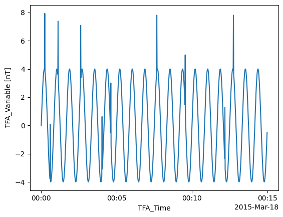
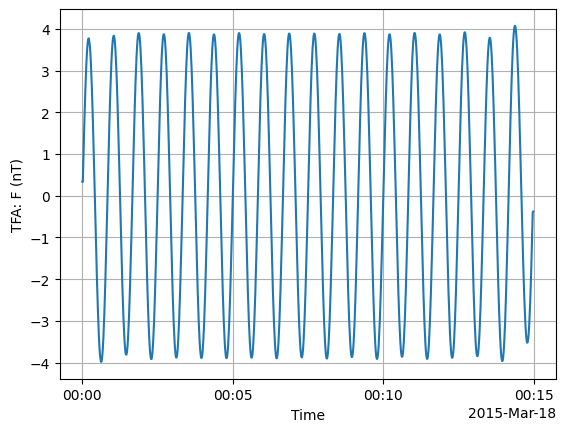
Let’s test the analysis with an artificial series, so we’ll replace the TFA_Variable with a time series of our choice, with a specific frequency of 40 mHz (i.e. 25 sec) and amplitude of 4 nT.

To test the cleaning we’ll add some random spikes as well.

# Get a test wave with the same length as the data, sampled at 1Hz
N = data["SW_OPER_MAGA_LR_1B"]["TFA_Variable"].shape[0]
test_wave = 4 * np.sin(2 * np.pi * np.arange(N) / 50)
# Create ten spikes at ten random locations
np.random.seed(0)
spike_locations = np.random.randint(
    0,
    N,
    10,
)
test_wave[spike_locations] = test_wave[spike_locations] + 4
# Overwrite the data with the test data
data["SW_OPER_MAGA_LR_1B"]["TFA_Variable"].data = test_wave

data["SW_OPER_MAGA_LR_1B"]["TFA_Variable"].plot.line(x="TFA_Time");

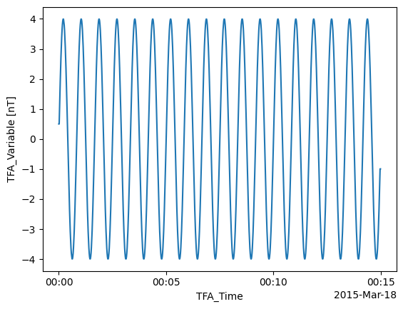
Let’s see the effect of the cleaning routine…

p2 = tfa.processes.Clean()
p2.set_config(
    window_size=10,
    method="iqr",
    multiplier=0.5,
)
p2(data)
data["SW_OPER_MAGA_LR_1B"]["TFA_Variable"].plot.line(x="TFA_Time");

… and the filtering…

p3 = tfa.processes.Filter()
p3.set_config(
    cutoff_frequency=10 / 1000,
)
p3(data)
tfa.plotting.time_series(data);

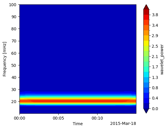
Next the wavelet transform is applied…

p4 = tfa.processes.Wavelet()
p4.set_config(
    min_frequency=10 / 1000,
    max_frequency=100 / 1000,
    dj=0.1,
)
p4(data);

tfa.plotting.spectrum(data, levels=np.linspace(0, 4, 20), log=False, extra_x=None);

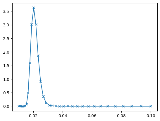
plt.plot(
    1 / data["SW_OPER_MAGA_LR_1B"]["scale"].data,
    data["SW_OPER_MAGA_LR_1B"]["wavelet_power"][:, int(N / 2)],
    "-x",
);