PAL-flavoured Datatree

The xarray Datatree is used as the core data structure for SwarmPAL. You can think of this like a file directory (a tree) which contains an arbitrary number of related xarray datasets. Data can be fetched from different resources (including VirES) and stored in a Datatree.

PalDataItem provides tools to construct an xarray.Dataset from different sources (VirES, HAPI, etc). create_paldata helps to construct a Datatree from a set of those datasets.

import datetime as dt

Fetching data

from swarmpal.io import create_paldata, PalDataItem

from VirES API

# Set of options which are passed to viresclient
data_params = dict(
    collection="SW_OPER_MAGA_LR_1B",
    measurements=["B_NEC"],
    models=["IGRF"],
    start_time="2016-01-01T00:00:00",
    end_time="2016-01-01T03:00:00",
    # start_time=dt.datetime(2016, 1, 1),  # Can use ISO string or datetime
    # end_time=dt.datetime(2016, 1, 1, 3),
    server_url="https://vires.services/ows",
    options=dict(asynchronous=False, show_progress=False),
)
# create_paldata takes an arbitrary number of args & kwargs
# If using args, dataset names will be used as tree names
# If using kwargs, user specifies the tree name/path
data = create_paldata(PalDataItem.from_vires(**data_params))
print(data)

<xarray.DataTree 'paldata'>
Group: /
└── Group: /SW_OPER_MAGA_LR_1B
        Dimensions:     (Timestamp: 10800, NEC: 3)
        Coordinates:
          * Timestamp   (Timestamp) datetime64[s] 86kB 2016-01-01 ... 2016-01-01T02:5...
          * NEC         (NEC) <U1 12B 'N' 'E' 'C'
        Data variables:
            Spacecraft  (Timestamp) object 86kB 'A' 'A' 'A' 'A' 'A' ... 'A' 'A' 'A' 'A'
            Radius      (Timestamp) float64 86kB 6.834e+06 6.834e+06 ... 6.833e+06
            Longitude   (Timestamp) float64 86kB 92.79 92.82 92.85 ... 41.83 41.83 41.83
            B_NEC       (Timestamp, NEC) float64 259kB -1.581e+03 ... -2.564e+04
            B_NEC_IGRF  (Timestamp, NEC) float64 259kB -1.578e+03 ... -2.564e+04
            Latitude    (Timestamp) float64 86kB -72.5 -72.56 -72.63 ... -44.97 -45.03
        Attributes:
            Sources:         ['SW_OPER_AUX_IGR_2__19000101T000000_20291231T235959_010...
            MagneticModels:  ['IGRF = IGRF(max_degree=13,min_degree=1)']
            AppliedFilters:  []
            PAL_meta:        {"analysis_window": ["2016-01-01T00:00:00", "2016-01-01T...

# Interactive view of the datatree
data

<xarray.DataTree 'paldata'>
Group: /
└── Group: /SW_OPER_MAGA_LR_1B
        Dimensions:     (Timestamp: 10800, NEC: 3)
        Coordinates:
          * Timestamp   (Timestamp) datetime64[s] 86kB 2016-01-01 ... 2016-01-01T02:5...
          * NEC         (NEC) <U1 12B 'N' 'E' 'C'
        Data variables:
            Spacecraft  (Timestamp) object 86kB 'A' 'A' 'A' 'A' 'A' ... 'A' 'A' 'A' 'A'
            Radius      (Timestamp) float64 86kB 6.834e+06 6.834e+06 ... 6.833e+06
            Longitude   (Timestamp) float64 86kB 92.79 92.82 92.85 ... 41.83 41.83 41.83
            B_NEC       (Timestamp, NEC) float64 259kB -1.581e+03 ... -2.564e+04
            B_NEC_IGRF  (Timestamp, NEC) float64 259kB -1.578e+03 ... -2.564e+04
            Latitude    (Timestamp) float64 86kB -72.5 -72.56 -72.63 ... -44.97 -45.03
        Attributes:
            Sources:         ['SW_OPER_AUX_IGR_2__19000101T000000_20291231T235959_010...
            MagneticModels:  ['IGRF = IGRF(max_degree=13,min_degree=1)']
            AppliedFilters:  []
            PAL_meta:        {"analysis_window": ["2016-01-01T00:00:00", "2016-01-01T...

xarray.DataTree

'paldata'

• /SW_OPER_MAGA_LR_1B(12)

  • Dimensions:
    • Timestamp: 10800
    • NEC: 3
  • Coordinates: (2)
    • Timestamp
      (Timestamp)
      datetime64[s]
      2016-01-01 ... 2016-01-01T02:59:59

      description :

      Time stamp

      array(['2016-01-01T00:00:00', '2016-01-01T00:00:01', '2016-01-01T00:00:02',..., '2016-01-01T02:59:57', '2016-01-01T02:59:58','2016-01-01T02:59:59'], shape=(10800,), dtype='datetime64[s]')

    • NEC
      (NEC)
      <U1
      'N' 'E' 'C'

      units :

      description :

      NEC frame - North, East, Centre (down)

      array(['N', 'E', 'C'], dtype='<U1')

  • Data variables: (6)
    • Spacecraft
      (Timestamp)
      object
      'A' 'A' 'A' 'A' ... 'A' 'A' 'A' 'A'

      units :

      -

      description :

      Spacecraft identifier (values: 'A', 'B', 'C' or '-' if not available).

      array(['A', 'A', 'A', ..., 'A', 'A', 'A'], shape=(10800,), dtype=object)

    • Radius
      (Timestamp)
      float64
      6.834e+06 6.834e+06 ... 6.833e+06

      units :

      m

      description :

      Position in ITRF - Radius

      array([6833853.11, 6833854.3 , 6833855.48, ..., 6832835.53, 6832839.08,6832842.63], shape=(10800,))

    • Longitude
      (Timestamp)
      float64
      92.79 92.82 92.85 ... 41.83 41.83

      units :

      deg

      description :

      Position in ITRF - Longitude

      array([92.7939649, 92.8226591, 92.8515848, ..., 41.8257328, 41.8274617,41.8292038], shape=(10800,))

    • B_NEC
      (Timestamp, NEC)
      float64
      -1.581e+03 ... -2.564e+04

      units :

      nT

      description :

      Magnetic field vector, NEC frame

      array([[ -1581.2973, -10494.2999, -45720.1707],[ -1607.9555, -10493.5039, -45716.6949],[ -1633.873 , -10491.8906, -45713.3837],...,[  9825.5389,  -8688.0132, -25614.0122],[  9821.3378,  -8698.109 , -25626.0085],[  9817.1922,  -8708.304 , -25638.1005]], shape=(10800, 3))

    • B_NEC_IGRF
      (Timestamp, NEC)
      float64
      -1.578e+03 ... -2.564e+04

      units :

      nT

      description :

      Magnetic field vector, NEC frame, calculated by the IGRF spherical harmonic model

      array([[ -1577.76166218, -10309.63589852, -45644.07256456],[ -1603.90449996, -10307.63142077, -45641.24499761],[ -1630.07857271, -10305.56776365, -45638.39192519],...,[  9837.46695817,  -8694.56699886, -25614.47699716],[  9833.31098636,  -8704.69655351, -25626.77067119],[  9829.18663666,  -8714.81373329, -25639.10587899]],shape=(10800, 3))

    • Latitude
      (Timestamp)
      float64
      -72.5 -72.56 ... -44.97 -45.03

      units :

      deg

      description :

      Position in ITRF - Latitude

      array([-72.4992236, -72.5623952, -72.6255613, ..., -44.9014651,-44.9653223, -45.0291791], shape=(10800,))

  • Attributes: (4)

    Sources :

    ['SW_OPER_AUX_IGR_2__19000101T000000_20291231T235959_0104', 'SW_OPER_MAGA_LR_1B_20160101T000000_20160101T235959_0701_MDR_MAG_LR']

    MagneticModels :

    ['IGRF = IGRF(max_degree=13,min_degree=1)']

    AppliedFilters :

    []

    PAL_meta :

    {"analysis_window": ["2016-01-01T00:00:00", "2016-01-01T03:00:00"], "magnetic_models": {"IGRF": "IGRF(max_degree=13,min_degree=1)"}, "config": {"pad_times": [], "collection": "SW_OPER_MAGA_LR_1B", "measurements": ["B_NEC"], "start_time": "2016-01-01T00:00:00", "end_time": "2016-01-01T03:00:00", "server_url": "https://vires.services/ows", "models": ["IGRF"], "auxiliaries": [], "sampling_step": null, "filters": [], "options": {"asynchronous": false, "show_progress": false}, "provider": "vires"}}

# Refer to a branch of the tree like:
data["SW_OPER_MAGA_LR_1B"]

<xarray.DataTree 'SW_OPER_MAGA_LR_1B'>
Group: /SW_OPER_MAGA_LR_1B
    Dimensions:     (Timestamp: 10800, NEC: 3)
    Coordinates:
      * Timestamp   (Timestamp) datetime64[s] 86kB 2016-01-01 ... 2016-01-01T02:5...
      * NEC         (NEC) <U1 12B 'N' 'E' 'C'
    Data variables:
        Spacecraft  (Timestamp) object 86kB 'A' 'A' 'A' 'A' 'A' ... 'A' 'A' 'A' 'A'
        Radius      (Timestamp) float64 86kB 6.834e+06 6.834e+06 ... 6.833e+06
        Longitude   (Timestamp) float64 86kB 92.79 92.82 92.85 ... 41.83 41.83 41.83
        B_NEC       (Timestamp, NEC) float64 259kB -1.581e+03 ... -2.564e+04
        B_NEC_IGRF  (Timestamp, NEC) float64 259kB -1.578e+03 ... -2.564e+04
        Latitude    (Timestamp) float64 86kB -72.5 -72.56 -72.63 ... -44.97 -45.03
    Attributes:
        Sources:         ['SW_OPER_AUX_IGR_2__19000101T000000_20291231T235959_010...
        MagneticModels:  ['IGRF = IGRF(max_degree=13,min_degree=1)']
        AppliedFilters:  []
        PAL_meta:        {"analysis_window": ["2016-01-01T00:00:00", "2016-01-01T...

xarray.DataTree

'SW_OPER_MAGA_LR_1B'

• Dimensions:
  • Timestamp: 10800
  • NEC: 3
• Coordinates: (2)
  • Timestamp
    (Timestamp)
    datetime64[s]
    2016-01-01 ... 2016-01-01T02:59:59

    description :

    Time stamp

    array(['2016-01-01T00:00:00', '2016-01-01T00:00:01', '2016-01-01T00:00:02',
           ..., '2016-01-01T02:59:57', '2016-01-01T02:59:58',
           '2016-01-01T02:59:59'], shape=(10800,), dtype='datetime64[s]')

  • NEC
    (NEC)
    <U1
    'N' 'E' 'C'

    units :

    description :

    NEC frame - North, East, Centre (down)

    array(['N', 'E', 'C'], dtype='<U1')

• Data variables: (6)
  • Spacecraft
    (Timestamp)
    object
    'A' 'A' 'A' 'A' ... 'A' 'A' 'A' 'A'

    units :

    -

    description :

    Spacecraft identifier (values: 'A', 'B', 'C' or '-' if not available).

    array(['A', 'A', 'A', ..., 'A', 'A', 'A'], shape=(10800,), dtype=object)

  • Radius
    (Timestamp)
    float64
    6.834e+06 6.834e+06 ... 6.833e+06

    units :

    m

    description :

    Position in ITRF - Radius

    array([6833853.11, 6833854.3 , 6833855.48, ..., 6832835.53, 6832839.08,
           6832842.63], shape=(10800,))

  • Longitude
    (Timestamp)
    float64
    92.79 92.82 92.85 ... 41.83 41.83

    units :

    deg

    description :

    Position in ITRF - Longitude

    array([92.7939649, 92.8226591, 92.8515848, ..., 41.8257328, 41.8274617,
           41.8292038], shape=(10800,))

  • B_NEC
    (Timestamp, NEC)
    float64
    -1.581e+03 ... -2.564e+04

    units :

    nT

    description :

    Magnetic field vector, NEC frame

    array([[ -1581.2973, -10494.2999, -45720.1707],
           [ -1607.9555, -10493.5039, -45716.6949],
           [ -1633.873 , -10491.8906, -45713.3837],
           ...,
           [  9825.5389,  -8688.0132, -25614.0122],
           [  9821.3378,  -8698.109 , -25626.0085],
           [  9817.1922,  -8708.304 , -25638.1005]], shape=(10800, 3))

  • B_NEC_IGRF
    (Timestamp, NEC)
    float64
    -1.578e+03 ... -2.564e+04

    units :

    nT

    description :

    Magnetic field vector, NEC frame, calculated by the IGRF spherical harmonic model

    array([[ -1577.76166218, -10309.63589852, -45644.07256456],
           [ -1603.90449996, -10307.63142077, -45641.24499761],
           [ -1630.07857271, -10305.56776365, -45638.39192519],
           ...,
           [  9837.46695817,  -8694.56699886, -25614.47699716],
           [  9833.31098636,  -8704.69655351, -25626.77067119],
           [  9829.18663666,  -8714.81373329, -25639.10587899]],
          shape=(10800, 3))

  • Latitude
    (Timestamp)
    float64
    -72.5 -72.56 ... -44.97 -45.03

    units :

    deg

    description :

    Position in ITRF - Latitude

    array([-72.4992236, -72.5623952, -72.6255613, ..., -44.9014651,
           -44.9653223, -45.0291791], shape=(10800,))

• Attributes: (4)

  Sources :

  ['SW_OPER_AUX_IGR_2__19000101T000000_20291231T235959_0104', 'SW_OPER_MAGA_LR_1B_20160101T000000_20160101T235959_0701_MDR_MAG_LR']

  MagneticModels :

  ['IGRF = IGRF(max_degree=13,min_degree=1)']

  AppliedFilters :

  []

  PAL_meta :

  {"analysis_window": ["2016-01-01T00:00:00", "2016-01-01T03:00:00"], "magnetic_models": {"IGRF": "IGRF(max_degree=13,min_degree=1)"}, "config": {"pad_times": [], "collection": "SW_OPER_MAGA_LR_1B", "measurements": ["B_NEC"], "start_time": "2016-01-01T00:00:00", "end_time": "2016-01-01T03:00:00", "server_url": "https://vires.services/ows", "models": ["IGRF"], "auxiliaries": [], "sampling_step": null, "filters": [], "options": {"asynchronous": false, "show_progress": false}, "provider": "vires"}}

# Note that the above is actually a Datatree object
# To get a view of the Dataset:
data["SW_OPER_MAGA_LR_1B"].ds

<xarray.DatasetView> Size: 950kB
Dimensions:     (Timestamp: 10800, NEC: 3)
Coordinates:
  * Timestamp   (Timestamp) datetime64[s] 86kB 2016-01-01 ... 2016-01-01T02:5...
  * NEC         (NEC) <U1 12B 'N' 'E' 'C'
Data variables:
    Spacecraft  (Timestamp) object 86kB 'A' 'A' 'A' 'A' 'A' ... 'A' 'A' 'A' 'A'
    Radius      (Timestamp) float64 86kB 6.834e+06 6.834e+06 ... 6.833e+06
    Longitude   (Timestamp) float64 86kB 92.79 92.82 92.85 ... 41.83 41.83 41.83
    B_NEC       (Timestamp, NEC) float64 259kB -1.581e+03 ... -2.564e+04
    B_NEC_IGRF  (Timestamp, NEC) float64 259kB -1.578e+03 ... -2.564e+04
    Latitude    (Timestamp) float64 86kB -72.5 -72.56 -72.63 ... -44.97 -45.03
Attributes:
    Sources:         ['SW_OPER_AUX_IGR_2__19000101T000000_20291231T235959_010...
    MagneticModels:  ['IGRF = IGRF(max_degree=13,min_degree=1)']
    AppliedFilters:  []
    PAL_meta:        {"analysis_window": ["2016-01-01T00:00:00", "2016-01-01T...

xarray.DatasetView

• Dimensions:
  • Timestamp: 10800
  • NEC: 3
• Coordinates: (2)
  • Timestamp
    (Timestamp)
    datetime64[s]
    2016-01-01 ... 2016-01-01T02:59:59

    description :

    Time stamp

    array(['2016-01-01T00:00:00', '2016-01-01T00:00:01', '2016-01-01T00:00:02',
           ..., '2016-01-01T02:59:57', '2016-01-01T02:59:58',
           '2016-01-01T02:59:59'], shape=(10800,), dtype='datetime64[s]')

  • NEC
    (NEC)
    <U1
    'N' 'E' 'C'

    units :

    description :

    NEC frame - North, East, Centre (down)

    array(['N', 'E', 'C'], dtype='<U1')

• Data variables: (6)
  • Spacecraft
    (Timestamp)
    object
    'A' 'A' 'A' 'A' ... 'A' 'A' 'A' 'A'

    units :

    -

    description :

    Spacecraft identifier (values: 'A', 'B', 'C' or '-' if not available).

    array(['A', 'A', 'A', ..., 'A', 'A', 'A'], shape=(10800,), dtype=object)

  • Radius
    (Timestamp)
    float64
    6.834e+06 6.834e+06 ... 6.833e+06

    units :

    m

    description :

    Position in ITRF - Radius

    array([6833853.11, 6833854.3 , 6833855.48, ..., 6832835.53, 6832839.08,
           6832842.63], shape=(10800,))

  • Longitude
    (Timestamp)
    float64
    92.79 92.82 92.85 ... 41.83 41.83

    units :

    deg

    description :

    Position in ITRF - Longitude

    array([92.7939649, 92.8226591, 92.8515848, ..., 41.8257328, 41.8274617,
           41.8292038], shape=(10800,))

  • B_NEC
    (Timestamp, NEC)
    float64
    -1.581e+03 ... -2.564e+04

    units :

    nT

    description :

    Magnetic field vector, NEC frame

    array([[ -1581.2973, -10494.2999, -45720.1707],
           [ -1607.9555, -10493.5039, -45716.6949],
           [ -1633.873 , -10491.8906, -45713.3837],
           ...,
           [  9825.5389,  -8688.0132, -25614.0122],
           [  9821.3378,  -8698.109 , -25626.0085],
           [  9817.1922,  -8708.304 , -25638.1005]], shape=(10800, 3))

  • B_NEC_IGRF
    (Timestamp, NEC)
    float64
    -1.578e+03 ... -2.564e+04

    units :

    nT

    description :

    Magnetic field vector, NEC frame, calculated by the IGRF spherical harmonic model

    array([[ -1577.76166218, -10309.63589852, -45644.07256456],
           [ -1603.90449996, -10307.63142077, -45641.24499761],
           [ -1630.07857271, -10305.56776365, -45638.39192519],
           ...,
           [  9837.46695817,  -8694.56699886, -25614.47699716],
           [  9833.31098636,  -8704.69655351, -25626.77067119],
           [  9829.18663666,  -8714.81373329, -25639.10587899]],
          shape=(10800, 3))

  • Latitude
    (Timestamp)
    float64
    -72.5 -72.56 ... -44.97 -45.03

    units :

    deg

    description :

    Position in ITRF - Latitude

    array([-72.4992236, -72.5623952, -72.6255613, ..., -44.9014651,
           -44.9653223, -45.0291791], shape=(10800,))

• Attributes: (4)

  Sources :

  ['SW_OPER_AUX_IGR_2__19000101T000000_20291231T235959_0104', 'SW_OPER_MAGA_LR_1B_20160101T000000_20160101T235959_0701_MDR_MAG_LR']

  MagneticModels :

  ['IGRF = IGRF(max_degree=13,min_degree=1)']

  AppliedFilters :

  []

  PAL_meta :

  {"analysis_window": ["2016-01-01T00:00:00", "2016-01-01T03:00:00"], "magnetic_models": {"IGRF": "IGRF(max_degree=13,min_degree=1)"}, "config": {"pad_times": [], "collection": "SW_OPER_MAGA_LR_1B", "measurements": ["B_NEC"], "start_time": "2016-01-01T00:00:00", "end_time": "2016-01-01T03:00:00", "server_url": "https://vires.services/ows", "models": ["IGRF"], "auxiliaries": [], "sampling_step": null, "filters": [], "options": {"asynchronous": false, "show_progress": false}, "provider": "vires"}}

swarmpal accessor

The behaviour of the datatree is extended by the addition of an “accessor” that adds functionality from SwarmPAL under the .swarmpal namespace, e.g.:

# Metadata related to the SwarmPAL framework
data.swarmpal.pal_meta

{'.': {},
 'SW_OPER_MAGA_LR_1B': {'analysis_window': ['2016-01-01T00:00:00',
   '2016-01-01T03:00:00'],
  'magnetic_models': {'IGRF': 'IGRF(max_degree=13,min_degree=1)'},
  'config': {'pad_times': [],
   'collection': 'SW_OPER_MAGA_LR_1B',
   'measurements': ['B_NEC'],
   'start_time': '2016-01-01T00:00:00',
   'end_time': '2016-01-01T03:00:00',
   'server_url': 'https://vires.services/ows',
   'models': ['IGRF'],
   'auxiliaries': [],
   'sampling_step': None,
   'filters': [],
   'options': {'asynchronous': False, 'show_progress': False},
   'provider': 'vires'}}}

data.swarmpal.magnetic_model_name

'IGRF'

The above properties are constructed from metadata which are stored within the datatree itself:

data["SW_OPER_MAGA_LR_1B"].attrs["PAL_meta"]

'{"analysis_window": ["2016-01-01T00:00:00", "2016-01-01T03:00:00"], "magnetic_models": {"IGRF": "IGRF(max_degree=13,min_degree=1)"}, "config": {"pad_times": [], "collection": "SW_OPER_MAGA_LR_1B", "measurements": ["B_NEC"], "start_time": "2016-01-01T00:00:00", "end_time": "2016-01-01T03:00:00", "server_url": "https://vires.services/ows", "models": ["IGRF"], "auxiliaries": [], "sampling_step": null, "filters": [], "options": {"asynchronous": false, "show_progress": false}, "provider": "vires"}}'

It is possible to add more complex methods that work on the datasets:

data["SW_OPER_MAGA_LR_1B"].swarmpal.magnetic_residual()

<xarray.DataArray (Timestamp: 10800, NEC: 3)> Size: 259kB
array([[  -3.53563782, -184.66400148,  -76.09813544],
       [  -4.05100004, -185.87247923,  -75.44990239],
       [  -3.79442729, -186.32283635,  -74.99177481],
       ...,
       [ -11.92805817,    6.55379886,    0.46479716],
       [ -11.97318636,    6.58755351,    0.76217119],
       [ -11.99443666,    6.50973329,    1.00537899]], shape=(10800, 3))
Coordinates:
  * Timestamp  (Timestamp) datetime64[s] 86kB 2016-01-01 ... 2016-01-01T02:59:59
  * NEC        (NEC) <U1 12B 'N' 'E' 'C'
Attributes:
    units:        nT
    description:  Magnetic field vector data-model residual, NEC frame

xarray.DataArray

• Timestamp: 10800
• NEC: 3

• -3.536 -184.7 -76.1 -4.051 -185.9 ... 6.588 0.7622 -11.99 6.51 1.005

  array([[  -3.53563782, -184.66400148,  -76.09813544],
         [  -4.05100004, -185.87247923,  -75.44990239],
         [  -3.79442729, -186.32283635,  -74.99177481],
         ...,
         [ -11.92805817,    6.55379886,    0.46479716],
         [ -11.97318636,    6.58755351,    0.76217119],
         [ -11.99443666,    6.50973329,    1.00537899]], shape=(10800, 3))

• Coordinates: (2)
  • Timestamp
    (Timestamp)
    datetime64[s]
    2016-01-01 ... 2016-01-01T02:59:59

    description :

    Time stamp

    array(['2016-01-01T00:00:00', '2016-01-01T00:00:01', '2016-01-01T00:00:02',
           ..., '2016-01-01T02:59:57', '2016-01-01T02:59:58',
           '2016-01-01T02:59:59'], shape=(10800,), dtype='datetime64[s]')

  • NEC
    (NEC)
    <U1
    'N' 'E' 'C'

    units :

    description :

    NEC frame - North, East, Centre (down)

    array(['N', 'E', 'C'], dtype='<U1')

• Attributes: (2)

  units :

  nT

  description :

  Magnetic field vector data-model residual, NEC frame

Defining and running a PalProcess

A process can be defined which will act on datatrees obtained as above. Define processes by subclassing the abstract PalProcess class.

from swarmpal.io import PalProcess

help(PalProcess)

Help on class PalProcess in module swarmpal.io._paldata:

class PalProcess(abc.ABC)
 |  PalProcess(config: 'dict | None' = None, active_tree: 'str' = '/', inplace: 'bool' = True)
 |  
 |  Abstract class to define processes to act on datatrees
 |  
 |  Method resolution order:
 |      PalProcess
 |      abc.ABC
 |      builtins.object
 |  
 |  Methods defined here:
 |  
 |  __call__(self, datatree) -> 'DataTree'
 |      Run the process, defined in _call, to update the datatree
 |  
 |  __init__(self, config: 'dict | None' = None, active_tree: 'str' = '/', inplace: 'bool' = True)
 |      Initialize self.  See help(type(self)) for accurate signature.
 |  
 |  set_config(self, output_dataset: 'str' = '', **kwargs)
 |  
 |  ----------------------------------------------------------------------
 |  Readonly properties defined here:
 |  
 |  active_tree
 |      Defines which branch of the datatree will be used
 |  
 |  output_dataset
 |  
 |  process_name
 |  
 |  ----------------------------------------------------------------------
 |  Data descriptors defined here:
 |  
 |  __dict__
 |      dictionary for instance variables
 |  
 |  __weakref__
 |      list of weak references to the object
 |  
 |  config
 |      Dictionary that configures the process behaviour
 |  
 |  ----------------------------------------------------------------------
 |  Data and other attributes defined here:
 |  
 |  __abstractmethods__ = frozenset({'_call', 'process_name', 'set_config'...

Here is an example of defining a process. Still subject to change!

Three methods must be set:

• process_name identifies the process, and is used to update the "PAL_meta" attribute in the datatree when the process is applied.

• set_config takes keyword arguments and stores them as a dict in the config property.

• _call defines the behaviour of the process itself, and should accept the input datatree and return a modified datatree

When a process object is instantiated, the user optionally provides two arguments which are set as properties of the process

• active_tree (str) selects which branch of the tree is to be used

• config (dict) provides parameters to control the behaviour of the process

The config can also be provided using .set_config() after the process object is created. This enables the process to provide and document default configurations, as well allowing the IDE to provide hints for what configuration is available.

from xarray import Dataset, DataTree


class MyProcess(PalProcess):
    """Compute the first differences on a given variable"""

    @property
    def process_name(self):
        return "MyProcess"

    def set_config(
        self, dataset="SW_OPER_MAGA_LR_1B", parameter="B_NEC", output_dataset="PAL_OUT"
    ):
        super().set_config(
            dataset=dataset, parameter=parameter, output_dataset=output_dataset
        )

    def _call(self, datatree):
        # Identify inputs for algorithm
        subtree = datatree[f"{self.config.get('dataset')}"]
        dataset = subtree.ds
        parameter = self.config.get("parameter")
        # Apply the algorithm
        output_data = dataset[parameter].diff(dim="Timestamp")
        # Create an output dataset
        data_out = Dataset(
            data_vars={
                f"ddt ({parameter})": output_data,
            }
        )
        # Write the output into a new path in the datatree and return it
        datatree[self.output_dataset] = DataTree(dataset=data_out)
        return datatree

The process can now be created with some configuration:

process = MyProcess(
    config={"dataset": "SW_OPER_MAGA_LR_1B", "parameter": "B_NEC"},
)

…and there is a tool to apply this process to the datatree:

data = data.swarmpal.apply(process)
print(data)

<xarray.DataTree 'paldata'>
Group: /
│   Attributes:
│       PAL_meta:  {"output_datasets": ["PAL_OUT"]}
├── Group: /SW_OPER_MAGA_LR_1B
│       Dimensions:     (Timestamp: 10800, NEC: 3)
│       Coordinates:
│         * Timestamp   (Timestamp) datetime64[s] 86kB 2016-01-01 ... 2016-01-01T02:5...
│         * NEC         (NEC) <U1 12B 'N' 'E' 'C'
│       Data variables:
│           Spacecraft  (Timestamp) object 86kB 'A' 'A' 'A' 'A' 'A' ... 'A' 'A' 'A' 'A'
│           Radius      (Timestamp) float64 86kB 6.834e+06 6.834e+06 ... 6.833e+06
│           Longitude   (Timestamp) float64 86kB 92.79 92.82 92.85 ... 41.83 41.83 41.83
│           B_NEC       (Timestamp, NEC) float64 259kB -1.581e+03 ... -2.564e+04
│           B_NEC_IGRF  (Timestamp, NEC) float64 259kB -1.578e+03 ... -2.564e+04
│           Latitude    (Timestamp) float64 86kB -72.5 -72.56 -72.63 ... -44.97 -45.03
│       Attributes:
│           Sources:         ['SW_OPER_AUX_IGR_2__19000101T000000_20291231T235959_010...
│           MagneticModels:  ['IGRF = IGRF(max_degree=13,min_degree=1)']
│           AppliedFilters:  []
│           PAL_meta:        {"analysis_window": ["2016-01-01T00:00:00", "2016-01-01T...
└── Group: /PAL_OUT
        Dimensions:      (Timestamp: 10799, NEC: 3)
        Coordinates:
          * Timestamp    (Timestamp) datetime64[s] 86kB 2016-01-01T00:00:01 ... 2016-...
          * NEC          (NEC) <U1 12B 'N' 'E' 'C'
        Data variables:
            ddt (B_NEC)  (Timestamp, NEC) float64 259kB -26.66 0.796 ... -10.19 -12.09
        Attributes:
            PAL_meta:  {"MyProcess": {"output_dataset": "PAL_OUT", "dataset": "SW_OPE...

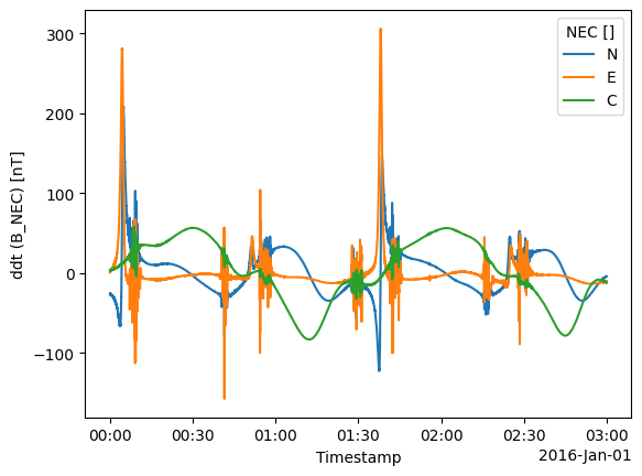
The resulting data can be interrogated with the usual tools (in this case we added a new dataset to the tree under "/output"):

data["PAL_OUT"].ds["ddt (B_NEC)"].plot.line(x="Timestamp");

… and the datatree carries with it the metadata about the process which has been applied:

data.swarmpal.pal_meta

{'.': {'output_datasets': ['PAL_OUT']},
 'SW_OPER_MAGA_LR_1B': {'analysis_window': ['2016-01-01T00:00:00',
   '2016-01-01T03:00:00'],
  'magnetic_models': {'IGRF': 'IGRF(max_degree=13,min_degree=1)'},
  'config': {'pad_times': [],
   'collection': 'SW_OPER_MAGA_LR_1B',
   'measurements': ['B_NEC'],
   'start_time': '2016-01-01T00:00:00',
   'end_time': '2016-01-01T03:00:00',
   'server_url': 'https://vires.services/ows',
   'models': ['IGRF'],
   'auxiliaries': [],
   'sampling_step': None,
   'filters': [],
   'options': {'asynchronous': False, 'show_progress': False},
   'provider': 'vires'}},
 'PAL_OUT': {'MyProcess': {'output_dataset': 'PAL_OUT',
   'dataset': 'SW_OPER_MAGA_LR_1B',
   'parameter': 'B_NEC'}}}

More tricks with create_paldata

Fetching data from HAPI

Two differences from using VirES:

• Parameters follow the scheme in hapiclient
  Example: http://hapi-server.org/servers/#server=VirES-for-Swarm&dataset=SW_OPER_MAGA_LR_1B&parameters=B_NEC&start=2016-01-01T00:00:00&stop=2016-01-01T03:00:00&return=script&format=python

• The output dataset is not identical to that retrieved from VirES (variables and their content are the same, but less metadata etc)

data_params = dict(
    server="https://vires.services/hapi",
    dataset="SW_OPER_MAGA_LR_1B",
    parameters="B_NEC",
    start="2016-01-01T00:00:00",
    stop="2016-01-01T03:00:00",
)
data_hapi = create_paldata(alpha_hapi=PalDataItem.from_hapi(**data_params))
print(data_hapi)

<xarray.DataTree 'paldata'>
Group: /
└── Group: /alpha_hapi
        Dimensions:    (Timestamp: 10800, B_NEC_dim1: 3)
        Coordinates:
          * Timestamp  (Timestamp) datetime64[us] 86kB 2016-01-01 ... 2016-01-01T02:5...
        Dimensions without coordinates: B_NEC_dim1
        Data variables:
            B_NEC      (Timestamp, B_NEC_dim1) float64 259kB -1.581e+03 ... -2.564e+04
        Attributes:
            PAL_meta:  {"analysis_window": ["2016-01-01T00:00:00", "2016-01-01T03:00:...

Time padding

A tuple of timedelta can be given as an extra parameter. This extends the retrieved time interval, while storing the original time interval in "analysis_window" within the "Pal_meta" attribute.

data_params = dict(
    server="https://vires.services/hapi",
    dataset="SW_OPER_MAGA_LR_1B",
    parameters="B_NEC",
    start="2016-01-01T00:00:00",
    stop="2016-01-01T03:00:00",
    pad_times=(dt.timedelta(hours=1), dt.timedelta(hours=1)),
)
data_hapi = create_paldata(alpha_hapi=PalDataItem.from_hapi(**data_params))
print(data_hapi)

<xarray.DataTree 'paldata'>
Group: /
└── Group: /alpha_hapi
        Dimensions:    (Timestamp: 18000, B_NEC_dim1: 3)
        Coordinates:
          * Timestamp  (Timestamp) datetime64[us] 144kB 2015-12-31T23:00:00 ... 2016-...
        Dimensions without coordinates: B_NEC_dim1
        Data variables:
            B_NEC      (Timestamp, B_NEC_dim1) float64 432kB 2.08e+04 ... 4.618e+04
        Attributes:
            PAL_meta:  {"analysis_window": ["2016-01-01T00:00:00", "2016-01-01T03:00:...