Intro to the TFA tool and the Wavelet Transform#

Imports:

import datetime as dt

import matplotlib.pyplot as plt
import numpy as np

import swarmpal.toolboxes.tfa.tfa_processor as tfa

Provide values for the parameters of the analysis. The dataset can be chosen from one of the compatible magnetic data collections, and the var is a VirES-compatible variable string (see viresclient for more information). The “start” and “end” times must be given as a datetime object. If the data are required as they are, set the remove_chaos_model parameter to False. Otherwise, if the inputs are magnetic field data and the analysis requires subtraction of the model field, set the parameter to True.

dataset = "SW_OPER_MAGA_LR_1B"
var = "F"
remove_chaos_model = False
time_start = dt.datetime(2015, 3, 18)
time_end = dt.datetime(2015, 3, 18, 0, 15, 0)

Now run the TfaInput to retrieve the selected data.

inputs = tfa.TfaInput(
    collection=dataset,
    start_time=time_start,
    end_time=time_end,
    initialise=True,
    varname=var,
    sampling_time="PT1S",
    remove_chaos=remove_chaos_model,
)

# inputs.to_file('using_tfa.nc')
# inputs.initialise('using_tfa.nc')

The data now contains everything we need to start the processing. This data is contained in the .xarray attribute:

Let’s first test the analysis with an artificial series, so we’ll replace the F variable with a time series of our choice, with a specific frequency of 40 mHz (i.e. 25 sec) and amplitude of 4 nT.

To test the cleaning we’ll add some random spikes as well

N = inputs.xarray["F"].shape[0]  # get the length of the data
test_wave = 4 * np.sin(2 * np.pi * np.arange(N) / 50)
# test_wave = np.ones(N)

# create ten spikes at ten random locations
spike_locations = np.random.randint(0, 1000, 10) + int(N / 2) - 500
test_wave[spike_locations] = test_wave[spike_locations] + 4
inputs.xarray["F"].data = test_wave

To use the processing capabilities of TFA we create a TfaProcessor object, that contains the variable of choice.

processor = tfa.TfaProcessor(inputs, active_variable={"varname": var})

processor.plotX()

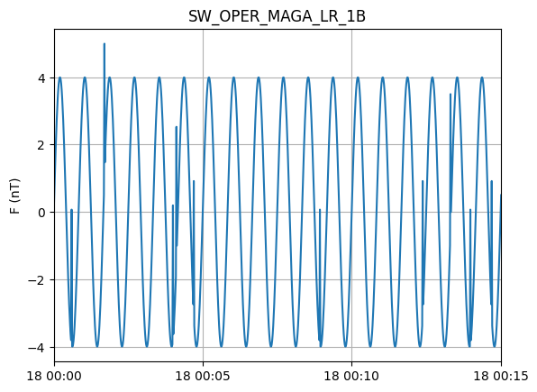
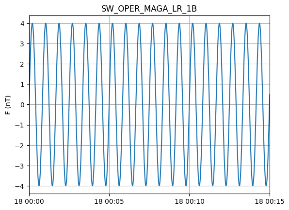
../../_images/26ceb92c3e870c6a94ef67fa3090f4128c734fc5d1a8f3b992dae579a758829b.png

To perform cleaning on the data, we initialize a Cleaning object with the parameters of our choice and then apply it on the data with the TfaProcessor apply() function. The active variable series can be plotted by means of the plotX() function.

c = tfa.Cleaning()
processor.apply(c)
processor.plotX()

../../_images/73e754deb2359dd0e34d278d2e6dda1496bda7add5f8de576a1ab69f58c7a404.png

Similarly, the filtering can be performed by first initializing a Filtering object with the parameters of our choosing and the applying in on the data.

f = tfa.Filtering()
processor.apply(f)

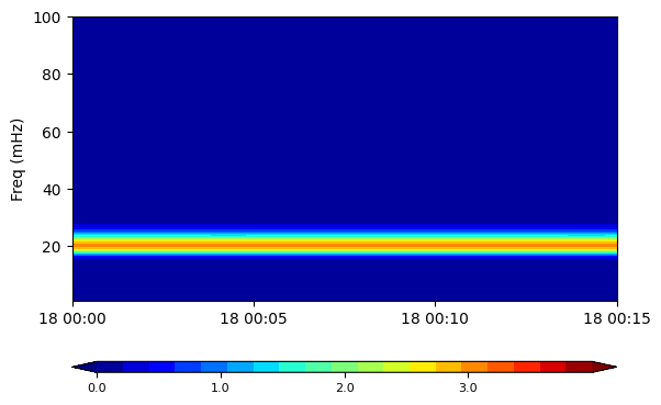
In the same way, the wavelet transform is applied

w = tfa.Wavelet()
processor.apply(w)

The result of the wavelet can be visualized by means of the image() function. Set the log parameter to True to plot the log-10 of the results or False to plot them as they are. The optional parameter cbar_lims can be set to specify the limits of the colorbar for the spectral plot.

processor.image(log=False, cbar_lims=[0, 4])

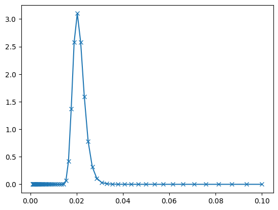
../../_images/e2b3e4ea7619dd868f04e54643cdac10282ceed53172f7aa5cefc55ef959d5d0.png

plt.plot(
    1 / processor.input_data.xarray["scale"].data,
    processor.input_data.xarray["wavelet_power"][:, int(N / 2)],
    "-x",
)

[<matplotlib.lines.Line2D at 0x7f54010d40d0>]

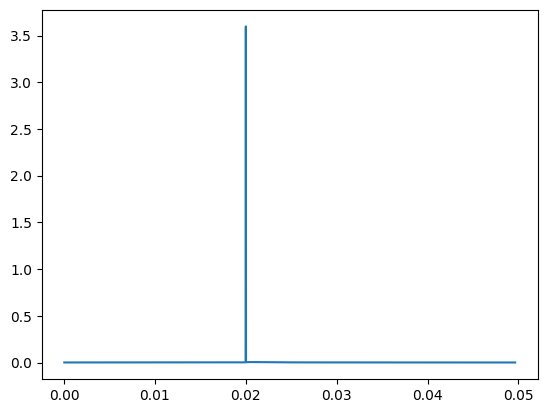
../../_images/d501237079be27162d2ce3974c7ae197ac302984b6b11e82e21ed6a2d2058384.png

fft_freq = np.arange(1, 2190) / N
F = np.abs(np.fft.fft(processor.input_data.xarray["X"].data)[1:2190]) / (N / 2)
plt.plot(fft_freq, F)

[<matplotlib.lines.Line2D at 0x7f5401051100>]

../../_images/2db9b5d78d996fd7ca61d6402292031cdd95da0c664da9e756b1c18a02457b9b.png

(
    np.sum(processor.input_data.xarray["wavelet_power"].data[:, int(N / 2)]),
    np.sum(F**2),
)

(12.959744228575715, 12.941911738953591)

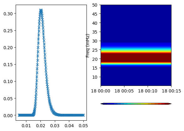
The same result holds even if one changes the frequency resolution.

w = tfa.Wavelet(
    {
        "Min_Scale": 1000 / 50,
        "Max_Scale": 1000 / 5,
        "dj": 0.01,
    }
)
processor.apply(w)
plt.subplot(1, 2, 1)
plt.plot(
    1 / processor.input_data.xarray["scale"].data,
    processor.input_data.xarray["wavelet_power"][:, int(N / 2)],
    "-x",
)
plt.subplot(1, 2, 2)
processor.image(log=False, cbar_lims=[0, 0.2])
np.sum(processor.input_data.xarray["wavelet_power"].data[:, int(N / 2)])

12.9597414132198

../../_images/6c8a198924ab58a8bb462610d12269fa9b88d52823bebe7b263f8db057d4b8bb.png

SwarmPAL

Intro to the TFA tool and the Wavelet Transform

Intro to the TFA tool and the Wavelet Transform#