TFA: Time-Frequency Analysis
Contents
TFA: Time-Frequency Analysis#
An overview of usage of the TFA toolbox. (To be separated out into different notebooks as before, overwriting those old ones)
%load_ext autoreload
%autoreload 2
import datetime as dt
import matplotlib.pyplot as plt
import numpy as np

from swarmpal.io import create_paldata, PalDataItem
from swarmpal.toolboxes import tfa
MAGx_LR example#
Fetching data#
data_params = dict(
    collection="SW_OPER_MAGA_LR_1B",
    measurements=["B_NEC", "F"],
    models=["Model='CHAOS-Core'+'CHAOS-Static'"],
    auxiliaries=["QDLat", "MLT"],
    start_time=dt.datetime(2015, 3, 14),
    end_time=dt.datetime(2015, 3, 14, 3, 59, 59),
    pad_times=(dt.timedelta(hours=3), dt.timedelta(hours=3)),
    server_url="https://vires.services/ows",
    options=dict(asynchronous=False, show_progress=False),
)
data = create_paldata(PalDataItem.from_vires(**data_params))
print(data)
DataTree('paldata', parent=None)
└── DataTree('SW_OPER_MAGA_LR_1B')
        Dimensions:      (Timestamp: 35999, NEC: 3)
        Coordinates:
          * Timestamp    (Timestamp) datetime64[ns] 2015-03-13T21:00:00 ... 2015-03-1...
          * NEC          (NEC) <U1 'N' 'E' 'C'
        Data variables:
            Spacecraft   (Timestamp) object 'A' 'A' 'A' 'A' 'A' ... 'A' 'A' 'A' 'A' 'A'
            Radius       (Timestamp) float64 6.835e+06 6.835e+06 ... 6.83e+06 6.83e+06
            Latitude     (Timestamp) float64 1.825 1.889 1.953 ... 34.16 34.1 34.03
            B_NEC_Model  (Timestamp, NEC) float64 2.177e+04 -4.168e+03 ... 2.571e+04
            QDLat        (Timestamp) float64 -9.028 -8.964 -8.9 ... 27.26 27.18 27.11
            F            (Timestamp) float64 2.354e+04 2.355e+04 ... 3.466e+04 3.464e+04
            MLT          (Timestamp) float64 19.82 19.82 19.82 ... 7.813 7.813 7.813
            B_NEC        (Timestamp, NEC) float64 2.175e+04 -4.166e+03 ... 2.572e+04
            Longitude    (Timestamp) float64 -15.47 -15.47 -15.47 ... 12.1 12.1 12.1
            F_Model      (Timestamp) float64 2.357e+04 2.357e+04 ... 3.466e+04 3.464e+04
        Attributes:
            Sources:         ['CHAOS-7_static.shc', 'SW_OPER_MAGA_LR_1B_20150313T0000...
            MagneticModels:  ["Model = 'CHAOS-Core'(max_degree=20,min_degree=1) + 'CH...
            AppliedFilters:  []
            PAL_meta:        {"analysis_window": ["2015-03-14T00:00:00", "2015-03-14T...
Applying processes#
TFA: Preprocess#
p1 = tfa.processes.Preprocess()
p1.set_config(
    dataset="SW_OPER_MAGA_LR_1B",
    active_variable="B_MFA",
    active_component=2,
    sampling_rate=1,
    remove_model=True,
    convert_to_mfa=True,
)
p1(data)
print(data)
DataTree('paldata', parent=None)
│   Dimensions:  ()
│   Data variables:
│       *empty*
│   Attributes:
│       PAL_meta:  {"TFA_Preprocess": {"dataset": "SW_OPER_MAGA_LR_1B", "timevar"...
└── DataTree('SW_OPER_MAGA_LR_1B')
        Dimensions:          (Timestamp: 35999, NEC: 3, MFA: 3, TFA_Time: 35999)
        Coordinates:
          * Timestamp        (Timestamp) datetime64[ns] 2015-03-13T21:00:00 ... 2015-...
          * NEC              (NEC) <U1 'N' 'E' 'C'
          * MFA              (MFA) int64 0 1 2
          * TFA_Time         (TFA_Time) datetime64[ns] 2015-03-13T21:00:00 ... 2015-0...
        Data variables: (12/13)
            Spacecraft       (Timestamp) object 'A' 'A' 'A' 'A' 'A' ... 'A' 'A' 'A' 'A'
            Radius           (Timestamp) float64 6.835e+06 6.835e+06 ... 6.83e+06
            Latitude         (Timestamp) float64 1.825 1.889 1.953 ... 34.16 34.1 34.03
            B_NEC_Model      (Timestamp, NEC) float64 2.177e+04 -4.168e+03 ... 2.571e+04
            QDLat            (Timestamp) float64 -9.028 -8.964 -8.9 ... 27.18 27.11
            F                (Timestamp) float64 2.354e+04 2.355e+04 ... 3.464e+04
            ...               ...
            B_NEC            (Timestamp, NEC) float64 2.175e+04 -4.166e+03 ... 2.572e+04
            Longitude        (Timestamp) float64 -15.47 -15.47 -15.47 ... 12.1 12.1 12.1
            F_Model          (Timestamp) float64 2.357e+04 2.357e+04 ... 3.464e+04
            B_NEC_res_Model  (Timestamp, NEC) float64 -24.7 2.017 4.414 ... -4.758 10.28
            B_MFA            (Timestamp, MFA) float64 4.208 -2.663 ... -4.483 0.6429
            TFA_Variable     (TFA_Time) float64 -24.67 -24.66 -24.68 ... 0.6687 0.6429
        Attributes:
            Sources:         ['CHAOS-7_static.shc', 'SW_OPER_MAGA_LR_1B_20150313T0000...
            MagneticModels:  ["Model = 'CHAOS-Core'(max_degree=20,min_degree=1) + 'CH...
            AppliedFilters:  []
            PAL_meta:        {"analysis_window": ["2015-03-14T00:00:00", "2015-03-14T...
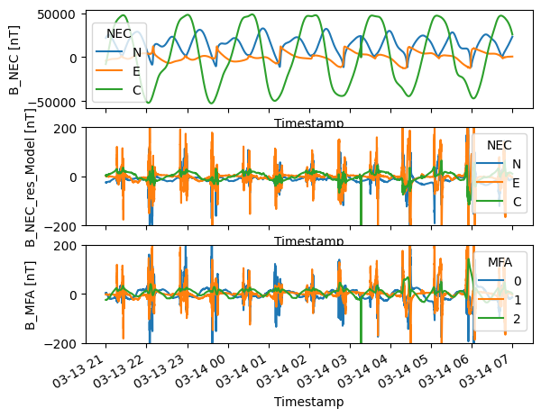
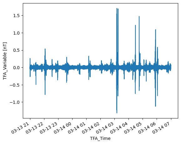
This data has been extended to include B_NEC_res_Model, B_MFA, and TFA_Variable. These can be inspected with the usual xarray/matplotlib tools
fig, axes = plt.subplots(3, 1, sharex=True)
data["SW_OPER_MAGA_LR_1B"]["B_NEC"].plot.line(x="Timestamp", ax=axes[0])
data["SW_OPER_MAGA_LR_1B"]["B_NEC_res_Model"].plot.line(x="Timestamp", ax=axes[1])
data["SW_OPER_MAGA_LR_1B"]["B_MFA"].plot.line(x="Timestamp", ax=axes[2])
axes[1].set_ylim(-200, 200)
axes[2].set_ylim(-200, 200);
data["SW_OPER_MAGA_LR_1B"]["TFA_Variable"].plot.line(x="TFA_Time");
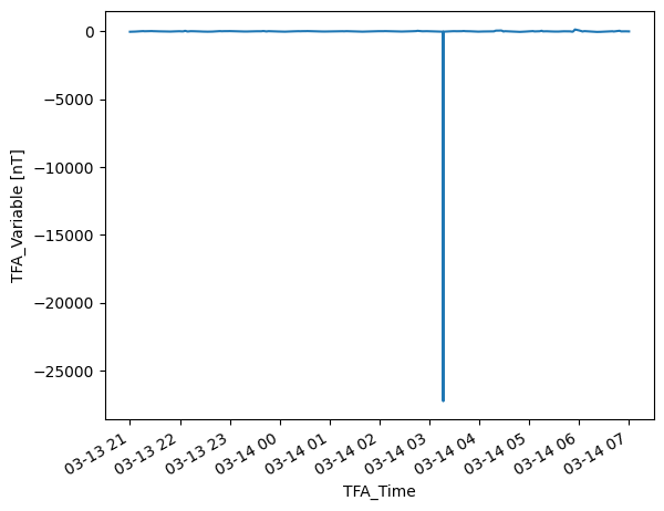
TFA: Clean#
p2 = tfa.processes.Clean()
p2.set_config(
    window_size=300,
    method="iqr",
    multiplier=1,
)
p2(data)
data["SW_OPER_MAGA_LR_1B"]["TFA_Variable"].plot.line(x="TFA_Time");
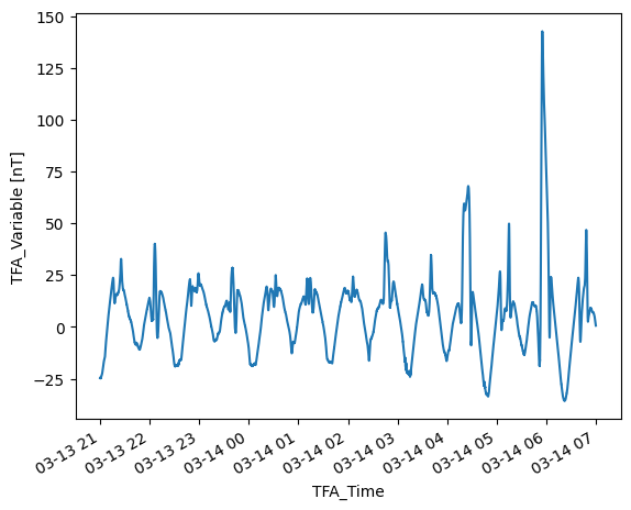
TFA: Filter#
p3 = tfa.processes.Filter()
p3.set_config(
    cutoff_frequency=20 / 1000,
)
p3(data)
data["SW_OPER_MAGA_LR_1B"]["TFA_Variable"].plot.line(x="TFA_Time");
TFA: Wavelet#
p4 = tfa.processes.Wavelet()
p4.set_config(
    min_frequency=20 / 1000,
    max_frequency=100 / 1000,
    dj=0.1,
)
p4(data)
print(data)
DataTree('paldata', parent=None)
│   Dimensions:  ()
│   Data variables:
│       *empty*
│   Attributes:
│       PAL_meta:  {"TFA_Preprocess": {"dataset": "SW_OPER_MAGA_LR_1B", "timevar"...
└── DataTree('SW_OPER_MAGA_LR_1B')
        Dimensions:          (Timestamp: 35999, NEC: 3, MFA: 3, TFA_Time: 35999,
                              scale: 24)
        Coordinates:
          * Timestamp        (Timestamp) datetime64[ns] 2015-03-13T21:00:00 ... 2015-...
          * NEC              (NEC) <U1 'N' 'E' 'C'
          * MFA              (MFA) int64 0 1 2
          * TFA_Time         (TFA_Time) datetime64[ns] 2015-03-13T21:00:00 ... 2015-0...
          * scale            (scale) float64 10.0 10.72 11.49 ... 42.87 45.95 49.25
        Data variables: (12/14)
            Spacecraft       (Timestamp) object 'A' 'A' 'A' 'A' 'A' ... 'A' 'A' 'A' 'A'
            Radius           (Timestamp) float64 6.835e+06 6.835e+06 ... 6.83e+06
            Latitude         (Timestamp) float64 1.825 1.889 1.953 ... 34.16 34.1 34.03
            B_NEC_Model      (Timestamp, NEC) float64 2.177e+04 -4.168e+03 ... 2.571e+04
            QDLat            (Timestamp) float64 -9.028 -8.964 -8.9 ... 27.18 27.11
            F                (Timestamp) float64 2.354e+04 2.355e+04 ... 3.464e+04
            ...               ...
            Longitude        (Timestamp) float64 -15.47 -15.47 -15.47 ... 12.1 12.1 12.1
            F_Model          (Timestamp) float64 2.357e+04 2.357e+04 ... 3.464e+04
            B_NEC_res_Model  (Timestamp, NEC) float64 -24.7 2.017 4.414 ... -4.758 10.28
            B_MFA            (Timestamp, MFA) float64 4.208 -2.663 ... -4.483 0.6429
            TFA_Variable     (TFA_Time) float64 -0.02522 -0.02383 ... 0.03256 0.07105
            wavelet_power    (scale, TFA_Time) float64 2.69e-05 2.458e-05 ... 9.341e-06
        Attributes:
            Sources:         ['CHAOS-7_static.shc', 'SW_OPER_MAGA_LR_1B_20150313T0000...
            MagneticModels:  ["Model = 'CHAOS-Core'(max_degree=20,min_degree=1) + 'CH...
            AppliedFilters:  []
            PAL_meta:        {"analysis_window": ["2015-03-14T00:00:00", "2015-03-14T...
Plotting#
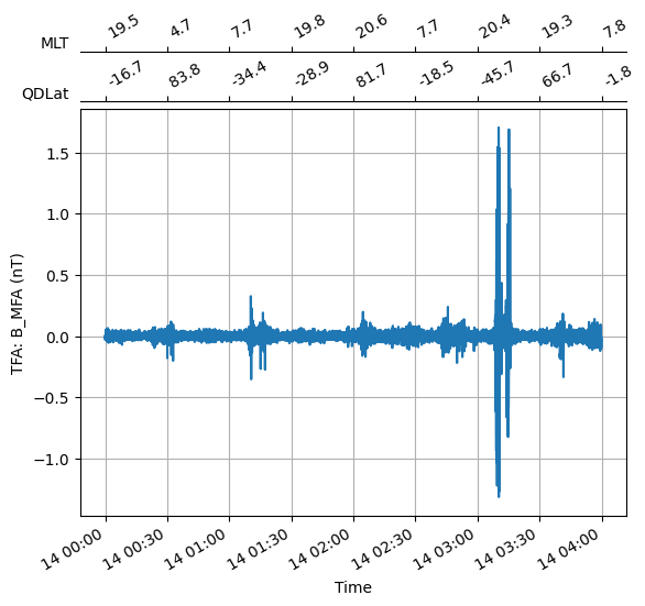
Special plotting functions are available under swarmpal.toolboxes.tfa.plotting. These accept the above datatree (data) as input.
Note that by default (see clip_times=True), these plots are restricted to the analysis window (the full time window minus the time pads added in the data request).
tfa.plotting.time_series(data)
(<Figure size 640x480 with 1 Axes>,
 <AxesSubplot: xlabel='Time', ylabel='TFA: B_MFA (nT)'>)
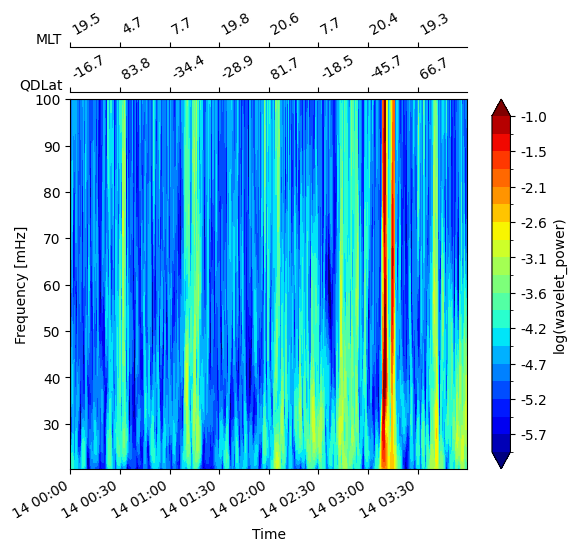
tfa.plotting.spectrum(data, levels=np.linspace(-6, -1, 20))
(<Figure size 640x480 with 2 Axes>,
 <AxesSubplot: xlabel='Time', ylabel='Frequency [mHz]'>)
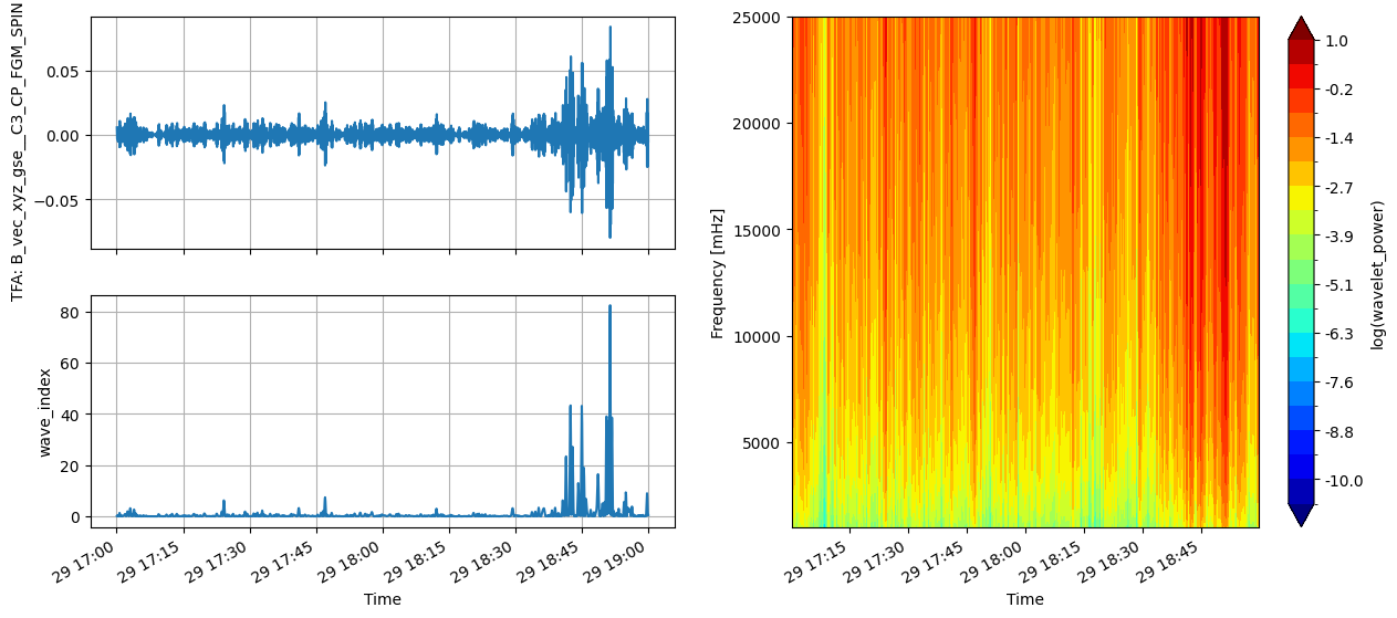
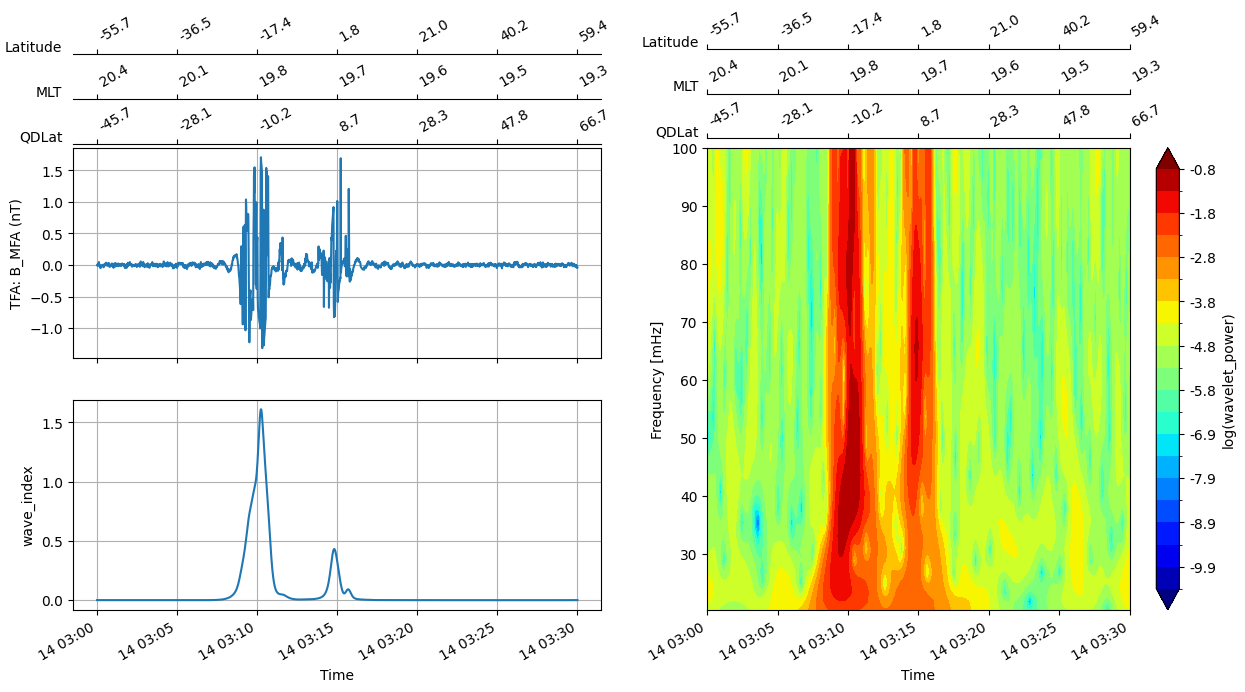
tfa.plotting.quicklook(data)
(<Figure size 1500x600 with 4 Axes>,
 (<AxesSubplot: ylabel='TFA: B_MFA (nT)'>,
  <AxesSubplot: xlabel='Time', ylabel='wave_index'>,
  <AxesSubplot: xlabel='Time', ylabel='Frequency [mHz]'>))
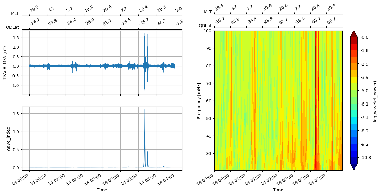
The plots can be configured with extra options like tlims (subsetting the time to plot), and extra_x (defining which extra x-axes to make).
tfa.plotting.quicklook(
    data,
    tlims=("2015-03-14T03:00:00", "2015-03-14T03:30:00"),
    extra_x=("QDLat", "MLT", "Latitude"),
)
(<Figure size 1500x600 with 4 Axes>,
 (<AxesSubplot: ylabel='TFA: B_MFA (nT)'>,
  <AxesSubplot: xlabel='Time', ylabel='wave_index'>,
  <AxesSubplot: xlabel='Time', ylabel='Frequency [mHz]'>))
MAGx_HR#
data_params = dict(
    collection="SW_OPER_MAGB_HR_1B",
    measurements=["B_NEC"],
    models=["Model='CHAOS-Core'+'CHAOS-Static'"],
    auxiliaries=["QDLat", "MLT"],
    start_time=dt.datetime(2015, 3, 14, 12, 5, 0),
    end_time=dt.datetime(2015, 3, 14, 12, 30, 0),
    pad_times=(dt.timedelta(minutes=10), dt.timedelta(minutes=10)),
    server_url="https://vires.services/ows",
    options=dict(asynchronous=False, show_progress=False),
)
data = create_paldata(PalDataItem.from_vires(**data_params))
p1 = tfa.processes.Preprocess()
p1.set_config(
    dataset="SW_OPER_MAGB_HR_1B",
    active_variable="B_NEC_res_Model",
    sampling_rate=50,
    remove_model=True,
    use_magnitude=True,
)
p2 = tfa.processes.Clean()
p2.set_config(
    window_size=300,
    method="iqr",
    multiplier=1,
)
p3 = tfa.processes.Filter()
p3.set_config(
    cutoff_frequency=0.1,
)
p4 = tfa.processes.Wavelet()
p4.set_config(
    min_frequency=1,
    max_frequency=25,
    dj=0.1,
)
p1(data)
p2(data)
p3(data)
p4(data);
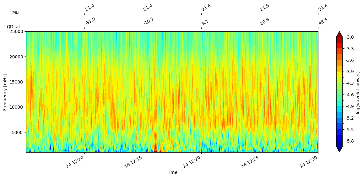
fig, ax = plt.subplots(1, 1, figsize=(15, 5))
tfa.plotting.spectrum(data, levels=np.linspace(-6, -3, 20), ax=ax)
(None, <AxesSubplot: xlabel='Time', ylabel='Frequency [mHz]'>)
EFIx_TCT#
data_params = dict(
    collection="SW_EXPT_EFIA_TCT02",
    measurements=["Ehx", "Ehy", "Ehz", "Quality_flags"],
    auxiliaries=["QDLat", "MLT"],
    start_time=dt.datetime(2015, 3, 14, 12, 5, 0),
    end_time=dt.datetime(2015, 3, 14, 12, 30, 0),
    pad_times=(dt.timedelta(hours=3), dt.timedelta(hours=3)),
    server_url="https://vires.services/ows",
    options=dict(asynchronous=False, show_progress=False),
)
data = create_paldata(PalDataItem.from_vires(**data_params))
p1 = tfa.processes.Preprocess()
p1.set_config(
    dataset="SW_EXPT_EFIA_TCT02",
    active_variable="Eh_XYZ",
    active_component=2,
    sampling_rate=2,
)
p2 = tfa.processes.Clean()
p2.set_config(
    window_size=300,
    method="iqr",
    multiplier=1,
)
p3 = tfa.processes.Filter()
p3.set_config(
    cutoff_frequency=20 / 1000,
)
p4 = tfa.processes.Wavelet()
p4.set_config(
    min_frequency=20 / 1000,
    max_frequency=200 / 1000,
    dj=0.1,
)
p1(data)
p2(data)
p3(data)
p4(data);
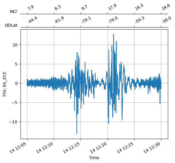
tfa.plotting.time_series(data)
(<Figure size 640x480 with 1 Axes>,
 <AxesSubplot: xlabel='Time', ylabel='TFA: Eh_XYZ'>)
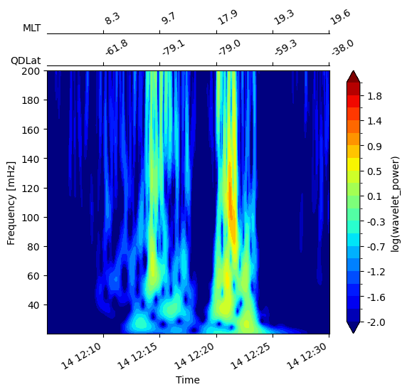
tfa.plotting.spectrum(data, levels=np.linspace(-2, 2, 20))
(<Figure size 640x480 with 2 Axes>,
 <AxesSubplot: xlabel='Time', ylabel='Frequency [mHz]'>)
AUX_OBS#
data_params = dict(
collection="SW_OPER_AUX_OBSM2_:HRN",
measurements=["B_NEC"],
models=["Model='CHAOS-Core'+'CHAOS-Static'"],
auxiliaries=["MLT"],
start_time=dt.datetime(2015, 3, 14, 0, 0, 0),
end_time=dt.datetime(2015, 3, 14, 23, 59, 59),
pad_times=(dt.timedelta(hours=3), dt.timedelta(hours=3)),
server_url="https://vires.services/ows",
options=dict(asynchronous=False, show_progress=False),
)
data = create_paldata(PalDataItem.from_vires(**data_params))
p1 = tfa.processes.Preprocess()
p1.set_config(
dataset="SW_OPER_AUX_OBSM2_:HRN",
active_variable="B_NEC_res_Model",
active_component=0,
sampling_rate=1 / 60,
remove_model=True,
)
p2 = tfa.processes.Clean()
p2.set_config(
window_size=10,
method="iqr",
multiplier=1,
)
p3 = tfa.processes.Filter()
p3.set_config(
cutoff_frequency=0.001,
)
p4 = tfa.processes.Wavelet()
p4.set_config(
min_scale=1000 / 8,
max_scale=1000 / 1,
dj=0.1,
)
p1(data)
p2(data)
p3(data)
p4(data)
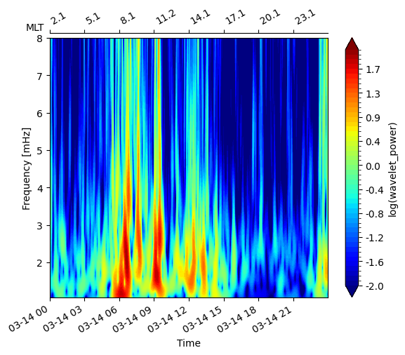
tfa.plotting.spectrum(data, levels=np.linspace(-2, 2))
Accessing INTERMAGNET and/or WDC data
Check usage terms at ftp://ftp.nerc-murchison.ac.uk/geomag/Swarm/AUX_OBS/minute/README
WARNING:swarmpal.toolboxes.tfa.plotting: Skipping QDLat: not available in data
(<Figure size 640x480 with 2 Axes>,
 <AxesSubplot: xlabel='Time', ylabel='Frequency [mHz]'>)
Cluster#
(Experimental) Note that these data are retrieved from the NASA CDAWeb HAPI server, and arguments to the data fetcher are supplied differently.
data_params = dict(
    server="https://cdaweb.gsfc.nasa.gov/hapi",
    dataset="C3_CP_FGM_SPIN",
    parameters="B_vec_xyz_gse__C3_CP_FGM_SPIN",
    start="2015-03-29T17:00:00",
    stop="2015-03-29T19:00:00",
    pad_times=(dt.timedelta(hours=3), dt.timedelta(hours=3)),
)
data = create_paldata(PalDataItem.from_hapi(**data_params))
print(data)
DataTree('paldata', parent=None)
└── DataTree('C3_CP_FGM_SPIN')
        Dimensions:                        (Time: 6839,
                                            B_vec_xyz_gse__C3_CP_FGM_SPIN_dim1: 3)
        Coordinates:
          * Time                           (Time) datetime64[ns] 2015-03-29T14:00:02....
        Dimensions without coordinates: B_vec_xyz_gse__C3_CP_FGM_SPIN_dim1
        Data variables:
            B_vec_xyz_gse__C3_CP_FGM_SPIN  (Time, B_vec_xyz_gse__C3_CP_FGM_SPIN_dim1) float64 ...
        Attributes:
            PAL_meta:  {"analysis_window": ["2015-03-29T17:00:00", "2015-03-29T19:00:...
/home/docs/checkouts/readthedocs.org/user_builds/swarmpal/envs/pre-cleanup/lib/python3.8/site-packages/hapiclient/hapitime.py:287: UserWarning: The argument 'infer_datetime_format' is deprecated and will be removed in a future version. A strict version of it is now the default, see https://pandas.pydata.org/pdeps/0004-consistent-to-datetime-parsing.html. You can safely remove this argument.
  Time = pandas.to_datetime(Time, infer_datetime_format=True).tz_convert(tzinfo).to_pydatetime()
p1 = tfa.processes.Preprocess()
p1.set_config(
    dataset="C3_CP_FGM_SPIN",
    timevar="Time",
    active_variable="B_vec_xyz_gse__C3_CP_FGM_SPIN",
    active_component=2,
    sampling_rate=1 / 4,
)
p2 = tfa.processes.Clean()
p2.set_config(
    window_size=300,
    method="iqr",
    multiplier=1,
)
p3 = tfa.processes.Filter()
p3.set_config(
    cutoff_frequency=0.1,
)
p4 = tfa.processes.Wavelet()
p4.set_config(
    min_frequency=1,
    max_frequency=25,
    dj=0.1,
)

data = data.pipe(p1).pipe(p2).pipe(p3).pipe(p4)
tfa.plotting.quicklook(data, extra_x=None);