TFA: Time-Frequency Analysis#
An introduction to the TFA toolbox. This gives a basic demonstration of a wavelet analysis applied to the MAGx_LR data (magnetic field 1Hz). For more details, see the following pages/notebooks.
import datetime as dt

from swarmpal.io import create_paldata, PalDataItem
from swarmpal.toolboxes import tfa
Fetching data#
create_paldata and PalDataItem.from_vires are used together to pull the desired data from VirES.
collection="SW_OPER_MAGA_LR_1B"selects the MAGx_LR dataset from Swarm Alphameasurements=["B_NEC"]selects the magnetic vector, B_NEC, which we will analyseWe provide a model choice with
models=["Model='CHAOS-Core'+'CHAOS-Static'"]. This can be changed to e.g.models=["Model=CHAOS"]which provides the full CHAOS model, including the magnetosphere. The string provided here is a VirES-compatible model string which specifies the chosen model (see viresclient for more information).The start and end times select the period we want to analyse
The
pad_timesoption supplies an extra padding of 3 hours of data before and after the analysis window, which prevents edge effects in the wavelet analysis
Running this code creates a DataTree object in the data variable. This contains all the data we will use in our analysis.
data = create_paldata(
    PalDataItem.from_vires(
        collection="SW_OPER_MAGA_LR_1B",
        measurements=["B_NEC"],
        models=["Model='CHAOS-Core'+'CHAOS-Static'"],
        auxiliaries=["QDLat", "MLT"],
        start_time=dt.datetime(2015, 3, 14),
        end_time=dt.datetime(2015, 3, 14, 3, 59, 59),
        pad_times=(dt.timedelta(hours=3), dt.timedelta(hours=3)),
        server_url="https://vires.services/ows",
        options=dict(asynchronous=False, show_progress=False),
    )
)
print(data)
<xarray.DataTree 'paldata'>
Group: /
└── Group: /SW_OPER_MAGA_LR_1B
        Dimensions:      (Timestamp: 35999, NEC: 3)
        Coordinates:
          * Timestamp    (Timestamp) datetime64[s] 288kB 2015-03-13T21:00:00 ... 2015...
          * NEC          (NEC) <U1 12B 'N' 'E' 'C'
        Data variables:
            Spacecraft   (Timestamp) object 288kB 'A' 'A' 'A' 'A' ... 'A' 'A' 'A' 'A'
            QDLat        (Timestamp) float64 288kB -9.028 -8.964 -8.899 ... 27.18 27.11
            Longitude    (Timestamp) float64 288kB -15.47 -15.47 -15.47 ... 12.1 12.1
            B_NEC        (Timestamp, NEC) float64 864kB 2.175e+04 ... 2.572e+04
            MLT          (Timestamp) float64 288kB 19.82 19.82 19.82 ... 7.813 7.813
            Radius       (Timestamp) float64 288kB 6.835e+06 6.835e+06 ... 6.83e+06
            B_NEC_Model  (Timestamp, NEC) float64 864kB 2.177e+04 ... 2.571e+04
            Latitude     (Timestamp) float64 288kB 1.825 1.889 1.953 ... 34.1 34.03
        Attributes:
            Sources:         ['CHAOS-8.1_static.shc', 'SW_OPER_MAGA_LR_1B_20150313T00...
            MagneticModels:  ["Model = 'CHAOS-Core'(max_degree=20,min_degree=1) + 'CH...
            AppliedFilters:  []
            PAL_meta:        {"analysis_window": ["2015-03-14T00:00:00", "2015-03-14T...
Applying processes#
Now we will apply some processes to our data. These are all available within the tfa submodule which we imported earlier.
TFA: Preprocess#
First we preprocess the data. To do this we use Preprocess, and, using .set_config, supply a configuration to control how that should behave. This will create a function that we can apply to the data - we will call this function p1 since it is the first process we will apply.
(Strictly speaking p1 is a special object rather than a regular function in Python, but has been made callable so that we can use it like p1(data) to apply it to data)
Some of the options are used here, but refer to the other demonstrations for more detail.
p1 = tfa.processes.Preprocess()
p1.set_config(
    # Identifies the data we are working with
    # (this dataset must be available in the DataTree above)
    dataset="SW_OPER_MAGA_LR_1B",
    # Selects the variable we want to process
    # B_NEC_res_Model is a special variable that is added to the data
    #   when we also specify remove_model=True
    active_variable="B_NEC_res_Model",
    # Selects which component (0, 1, 2) to process
    # With the NEC vectors, 2 will refer to the "C" (centre / downward) component
    active_component=2,
    # Identifies the sampling rate (in Hz) of the data
    sampling_rate=1,
    # Removes the magnetic model from the data
    # i.e. gets the data-model residual / perturbation
    remove_model=True,
)
Now we have a process p1, we can apply that to the data:
p1(data);
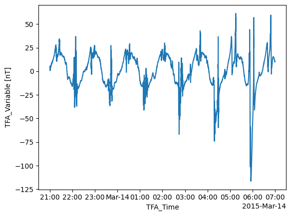
The preprocessing plays a number of roles but most importantly it sets a new array, TFA_Variable, in the data, which will be used in the following steps.
This data can be inspected directly using tools available through xarray:
data["PAL_TFA"]["TFA_Variable"]
<xarray.DataArray 'TFA_Variable' (TFA_Time: 35999)> Size: 288kB
array([4.48811864, 4.40565307, 4.29499901, ..., 9.99070629, 9.94805416,
       9.94434215], shape=(35999,))
Coordinates:
  * TFA_Time  (TFA_Time) datetime64[ns] 288kB 2015-03-13T21:00:00 ... 2015-03...
Attributes:
    units:        nT
description: Magnetic field vector data-model residual, NEC framedata["PAL_TFA"]["TFA_Variable"].plot.line(x="TFA_Time");
The TFA toolbox also provides a function to inspect the data, tfa.plotting.time_series:
tfa.plotting.time_series(data);
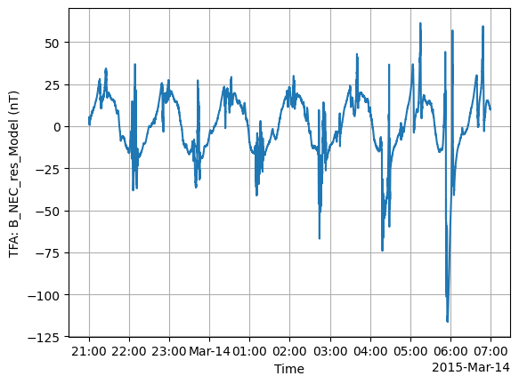
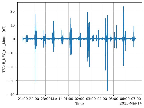
We can see an unphysical spike in the data. In this case we could have removed this bad data in the data request step (by filtering according to flag values), but here we will demonstrate the functionality of the TFA toolbox in removing this spike.
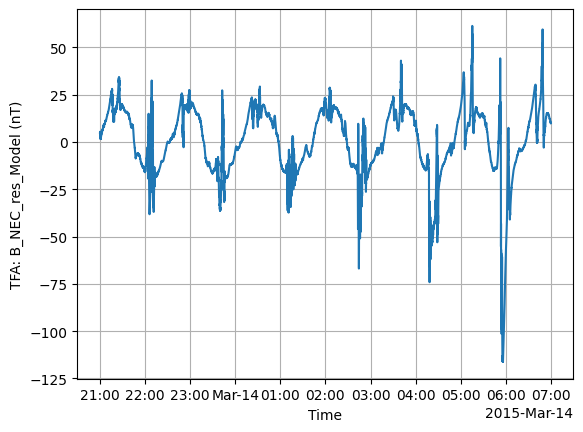
TFA: Clean#
Just as with Preprocess, there is Clean which provides a data cleaning function to remove outliers.
p2 = tfa.processes.Clean()
p2.set_config(
    window_size=300,
    method="iqr",
    multiplier=1,
)
p2(data)
tfa.plotting.time_series(data);
TFA: Filter#
Next we use Filter, which applies a high-pass filter to the data.
p3 = tfa.processes.Filter()
p3.set_config(
    cutoff_frequency=20 / 1000,
)
p3(data)
tfa.plotting.time_series(data);
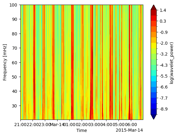
TFA: Wavelet#
Now we get to the most interesting part: applying a wavelet analysis.
p4 = tfa.processes.Wavelet()
p4.set_config(
    min_frequency=20 / 1000,
    max_frequency=100 / 1000,
    dj=0.1,
)
p4(data);
The results of the wavelet analysis are stored as a spectrum in a new wavelet_power array:
data["PAL_TFA"]["wavelet_power"]
<xarray.DataArray 'wavelet_power' (scale: 24, TFA_Time: 35999)> Size: 7MB
array([[0.000642  , 0.00066535, 0.00067605, ..., 0.00051215, 0.00056317,
        0.00060729],
       [0.00064137, 0.0006116 , 0.00056973, ..., 0.00066002, 0.00066468,
        0.00065887],
       [0.00067472, 0.00062239, 0.00056425, ..., 0.00078728, 0.00075765,
        0.00072005],
       ...,
       [0.02292635, 0.02340608, 0.02388445, ..., 0.02148465, 0.02196508,
        0.02244583],
       [0.02152357, 0.02197593, 0.02242583, ..., 0.02015701, 0.02061358,
        0.02106928],
       [0.01680465, 0.01716353, 0.01752023, ..., 0.01571916, 0.01608206,
        0.01644403]], shape=(24, 35999))
Coordinates:
  * scale     (scale) float64 192B 10.0 10.72 11.49 12.31 ... 42.87 45.95 49.25
* TFA_Time (TFA_Time) datetime64[ns] 288kB 2015-03-13T21:00:00 ... 2015-03...And we can view it with tfa.plotting.spectrum:
tfa.plotting.spectrum(data)
(<Figure size 640x480 with 2 Axes>,
 <Axes: xlabel='Time', ylabel='Frequency [mHz]'>)
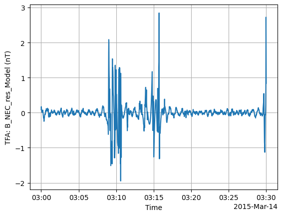
Plotting#
We showed basic usage of tfa.plotting.time_series and tfa.plotting.spectrum above. These have some extra options to control their behaviour. For example:
Adding extra x axes with
extra_xSelecting a specific time window with
tlims
tfa.plotting.time_series(
    data,
    extra_x=("QDLat", "MLT", "Latitude"),
    tlims=("2015-03-14T03:00:00", "2015-03-14T03:30:00"),
);
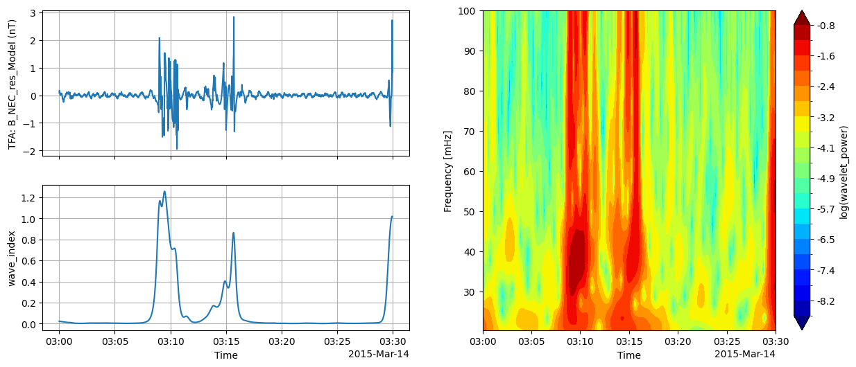
There is also a quicklook plot that combines the time series, spectrum, and wave power (from tfa.plotting.wave_index) into one figure:
tfa.plotting.quicklook(
    data,
    tlims=("2015-03-14T03:00:00", "2015-03-14T03:30:00"),
    extra_x=("QDLat", "MLT", "Latitude"),
);