DSECS: Dipolar Spherical Elementary Current Systems

For more information about the project and the technique, see:

• https://earth.esa.int/eogateway/activities/dsecs

• Vanhamäki, H., Maute, A., Alken, P. et al. Dipolar elementary current systems for ionospheric current reconstruction at low and middle latitudes. Earth Planets Space 72, 146 (2020). https://doi.org/10.1186/s40623-020-01284-1

import logging
import datetime as dt
from swarmpal.io import create_paldata, PalDataItem
from swarmpal.toolboxes import dsecs
import matplotlib.pyplot as plt

# To enable logging in the notebook, uncomment this line:
# logging.basicConfig(level=logging.INFO, force=True)

Fetching inputs to the toolbox

def data_params(spacecraft="A"):
    return dict(
        server_url="https://vires.services/ows",
        collection=f"SW_OPER_MAG{spacecraft}_LR_1B",
        measurements=["B_NEC"],
        models=["Model = CHAOS"],  # currently must use name "Model"
        auxiliaries=["QDLat"],
        start_time="2016-03-18T11:00:00",
        end_time="2016-03-18T14:00:00",
        filters=["OrbitDirection == 1"],  # Filters according to ascending passes
        options=dict(asynchronous=False, show_progress=False),
    )


data = create_paldata(
    PalDataItem.from_vires(**data_params("A")),
    PalDataItem.from_vires(**data_params("C")),
)

print(data)

<xarray.DataTree 'paldata'>
Group: /
├── Group: /SW_OPER_MAGA_LR_1B
│       Dimensions:      (Timestamp: 5506, NEC: 3)
│       Coordinates:
│         * Timestamp    (Timestamp) datetime64[s] 44kB 2016-03-18T11:00:00 ... 2016-...
│         * NEC          (NEC) <U1 12B 'N' 'E' 'C'
│       Data variables:
│           Spacecraft   (Timestamp) object 44kB 'A' 'A' 'A' 'A' 'A' ... 'A' 'A' 'A' 'A'
│           QDLat        (Timestamp) float64 44kB -68.58 -68.54 -68.5 ... 82.04 82.01
│           B_NEC        (Timestamp, NEC) float64 132kB 1.413e+04 ... 4.687e+04
│           Latitude     (Timestamp) float64 44kB -82.61 -82.55 -82.49 ... 87.35 87.35
│           Longitude    (Timestamp) float64 44kB -26.01 -25.83 -25.66 ... 48.7 50.09
│           B_NEC_Model  (Timestamp, NEC) float64 132kB 1.411e+04 ... 4.688e+04
│           Radius       (Timestamp) float64 44kB 6.832e+06 6.832e+06 ... 6.814e+06
│       Attributes:
│           Sources:         ['CHAOS-8.1_static.shc', 'SW_OPER_MAGA_LR_1B_20160318T00...
│           MagneticModels:  ["Model = 'CHAOS-Core'(max_degree=20,min_degree=1) + 'CH...
│           AppliedFilters:  ['OrbitDirection == 1']
│           PAL_meta:        {"analysis_window": ["2016-03-18T11:00:00", "2016-03-18T...
└── Group: /SW_OPER_MAGC_LR_1B
        Dimensions:      (Timestamp: 5500, NEC: 3)
        Coordinates:
          * Timestamp    (Timestamp) datetime64[s] 44kB 2016-03-18T11:00:00 ... 2016-...
          * NEC          (NEC) <U1 12B 'N' 'E' 'C'
        Data variables:
            Spacecraft   (Timestamp) object 44kB 'C' 'C' 'C' 'C' 'C' ... 'C' 'C' 'C' 'C'
            QDLat        (Timestamp) float64 44kB -68.47 -68.43 -68.39 ... 82.03 82.0
            B_NEC        (Timestamp, NEC) float64 132kB 1.412e+04 ... 4.688e+04
            Latitude     (Timestamp) float64 44kB -82.35 -82.29 -82.23 ... 87.35 87.35
            Longitude    (Timestamp) float64 44kB -23.86 -23.69 -23.54 ... 49.16 50.54
            B_NEC_Model  (Timestamp, NEC) float64 132kB 1.41e+04 ... 4.688e+04
            Radius       (Timestamp) float64 44kB 6.832e+06 6.832e+06 ... 6.814e+06
        Attributes:
            Sources:         ['CHAOS-8.1_static.shc', 'SW_OPER_MAGC_LR_1B_20160318T00...
            MagneticModels:  ["Model = 'CHAOS-Core'(max_degree=20,min_degree=1) + 'CH...
            AppliedFilters:  ['OrbitDirection == 1']
            PAL_meta:        {"analysis_window": ["2016-03-18T11:00:00", "2016-03-18T...

Applying the DSECS process

Preprocess

This initial process adds in Apex coordinates to the datasets.

p1 = dsecs.processes.Preprocess()
p1(data)
print(data)

<xarray.DataTree 'paldata'>
Group: /
│   Attributes:
│       PAL_meta:  {"output_datasets": ["DSECS_output"]}
├── Group: /SW_OPER_MAGA_LR_1B
│       Dimensions:        (Timestamp: 5506, NEC: 3)
│       Coordinates:
│         * Timestamp      (Timestamp) datetime64[s] 44kB 2016-03-18T11:00:00 ... 201...
│         * NEC            (NEC) <U1 12B 'N' 'E' 'C'
│       Data variables:
│           Spacecraft     (Timestamp) object 44kB 'A' 'A' 'A' 'A' ... 'A' 'A' 'A' 'A'
│           QDLat          (Timestamp) float64 44kB -68.58 -68.54 -68.5 ... 82.04 82.01
│           B_NEC          (Timestamp, NEC) float64 132kB 1.413e+04 ... 4.687e+04
│           Latitude       (Timestamp) float64 44kB -82.61 -82.55 -82.49 ... 87.35 87.35
│           Longitude      (Timestamp) float64 44kB -26.01 -25.83 -25.66 ... 48.7 50.09
│           B_NEC_Model    (Timestamp, NEC) float64 132kB 1.411e+04 ... 4.688e+04
│           Radius         (Timestamp) float64 44kB 6.832e+06 6.832e+06 ... 6.814e+06
│           ApexLatitude   (Timestamp) float64 44kB -69.37 -69.33 -69.29 ... 82.31 82.29
│           ApexLongitude  (Timestamp) float64 44kB 25.92 26.02 26.12 ... 155.1 155.5
│       Attributes:
│           Sources:         ['CHAOS-8.1_static.shc', 'SW_OPER_MAGA_LR_1B_20160318T00...
│           MagneticModels:  ["Model = 'CHAOS-Core'(max_degree=20,min_degree=1) + 'CH...
│           AppliedFilters:  ['OrbitDirection == 1']
│           PAL_meta:        {"analysis_window": ["2016-03-18T11:00:00", "2016-03-18T...
├── Group: /SW_OPER_MAGC_LR_1B
│       Dimensions:        (Timestamp: 5500, NEC: 3)
│       Coordinates:
│         * Timestamp      (Timestamp) datetime64[s] 44kB 2016-03-18T11:00:00 ... 201...
│         * NEC            (NEC) <U1 12B 'N' 'E' 'C'
│       Data variables:
│           Spacecraft     (Timestamp) object 44kB 'C' 'C' 'C' 'C' ... 'C' 'C' 'C' 'C'
│           QDLat          (Timestamp) float64 44kB -68.47 -68.43 -68.39 ... 82.03 82.0
│           B_NEC          (Timestamp, NEC) float64 132kB 1.412e+04 ... 4.688e+04
│           Latitude       (Timestamp) float64 44kB -82.35 -82.29 -82.23 ... 87.35 87.35
│           Longitude      (Timestamp) float64 44kB -23.86 -23.69 -23.54 ... 49.16 50.54
│           B_NEC_Model    (Timestamp, NEC) float64 132kB 1.41e+04 ... 4.688e+04
│           Radius         (Timestamp) float64 44kB 6.832e+06 6.832e+06 ... 6.814e+06
│           ApexLatitude   (Timestamp) float64 44kB -69.27 -69.23 -69.19 ... 82.3 82.28
│           ApexLongitude  (Timestamp) float64 44kB 26.81 26.91 27.01 ... 155.2 155.6
│       Attributes:
│           Sources:         ['CHAOS-8.1_static.shc', 'SW_OPER_MAGC_LR_1B_20160318T00...
│           MagneticModels:  ["Model = 'CHAOS-Core'(max_degree=20,min_degree=1) + 'CH...
│           AppliedFilters:  ['OrbitDirection == 1']
│           PAL_meta:        {"analysis_window": ["2016-03-18T11:00:00", "2016-03-18T...
└── Group: /DSECS_output
        Attributes:
            PAL_meta:  {"DSECS_Preprocess": {"output_dataset": "DSECS_output", "datas...

Analysis

This process performs the DSECS analysis. It currently takes about 3 minutes to process one pass over the mid-latitudes.

%%time
p2 = dsecs.processes.Analysis()
p2(data)

CPU times: user 4min 9s, sys: 2.63 s, total: 4min 11s
Wall time: 2min 53s

<xarray.DataTree 'paldata'>
Group: /
│   Attributes:
│       PAL_meta:  {"output_datasets": ["DSECS_output"]}
├── Group: /SW_OPER_MAGA_LR_1B
│       Dimensions:        (Timestamp: 5506, NEC: 3)
│       Coordinates:
│         * Timestamp      (Timestamp) datetime64[s] 44kB 2016-03-18T11:00:00 ... 201...
│         * NEC            (NEC) <U1 12B 'N' 'E' 'C'
│       Data variables:
│           Spacecraft     (Timestamp) object 44kB 'A' 'A' 'A' 'A' ... 'A' 'A' 'A' 'A'
│           QDLat          (Timestamp) float64 44kB -68.58 -68.54 -68.5 ... 82.04 82.01
│           B_NEC          (Timestamp, NEC) float64 132kB 1.413e+04 ... 4.687e+04
│           Latitude       (Timestamp) float64 44kB -82.61 -82.55 -82.49 ... 87.35 87.35
│           Longitude      (Timestamp) float64 44kB -26.01 -25.83 -25.66 ... 48.7 50.09
│           B_NEC_Model    (Timestamp, NEC) float64 132kB 1.411e+04 ... 4.688e+04
│           Radius         (Timestamp) float64 44kB 6.832e+06 6.832e+06 ... 6.814e+06
│           ApexLatitude   (Timestamp) float64 44kB -69.37 -69.33 -69.29 ... 82.31 82.29
│           ApexLongitude  (Timestamp) float64 44kB 25.92 26.02 26.12 ... 155.1 155.5
│       Attributes:
│           Sources:         ['CHAOS-8.1_static.shc', 'SW_OPER_MAGA_LR_1B_20160318T00...
│           MagneticModels:  ["Model = 'CHAOS-Core'(max_degree=20,min_degree=1) + 'CH...
│           AppliedFilters:  ['OrbitDirection == 1']
│           PAL_meta:        {"analysis_window": ["2016-03-18T11:00:00", "2016-03-18T...
├── Group: /SW_OPER_MAGC_LR_1B
│       Dimensions:        (Timestamp: 5500, NEC: 3)
│       Coordinates:
│         * Timestamp      (Timestamp) datetime64[s] 44kB 2016-03-18T11:00:00 ... 201...
│         * NEC            (NEC) <U1 12B 'N' 'E' 'C'
│       Data variables:
│           Spacecraft     (Timestamp) object 44kB 'C' 'C' 'C' 'C' ... 'C' 'C' 'C' 'C'
│           QDLat          (Timestamp) float64 44kB -68.47 -68.43 -68.39 ... 82.03 82.0
│           B_NEC          (Timestamp, NEC) float64 132kB 1.412e+04 ... 4.688e+04
│           Latitude       (Timestamp) float64 44kB -82.35 -82.29 -82.23 ... 87.35 87.35
│           Longitude      (Timestamp) float64 44kB -23.86 -23.69 -23.54 ... 49.16 50.54
│           B_NEC_Model    (Timestamp, NEC) float64 132kB 1.41e+04 ... 4.688e+04
│           Radius         (Timestamp) float64 44kB 6.832e+06 6.832e+06 ... 6.814e+06
│           ApexLatitude   (Timestamp) float64 44kB -69.27 -69.23 -69.19 ... 82.3 82.28
│           ApexLongitude  (Timestamp) float64 44kB 26.81 26.91 27.01 ... 155.2 155.6
│       Attributes:
│           Sources:         ['CHAOS-8.1_static.shc', 'SW_OPER_MAGC_LR_1B_20160318T00...
│           MagneticModels:  ["Model = 'CHAOS-Core'(max_degree=20,min_degree=1) + 'CH...
│           AppliedFilters:  ['OrbitDirection == 1']
│           PAL_meta:        {"analysis_window": ["2016-03-18T11:00:00", "2016-03-18T...
└── Group: /DSECS_output
    │   Attributes:
    │       PAL_meta:  {"DSECS_Preprocess": {"output_dataset": "DSECS_output", "datas...
    ├── Group: /DSECS_output/0
    │   ├── Group: /DSECS_output/0/currents
    │   │       Dimensions:      (x: 160, y: 7)
    │   │       Coordinates:
    │   │           Longitude    (x, y) float64 9kB 348.4 349.1 349.8 ... 350.5 351.2 351.9
    │   │           Latitude     (x, y) float64 9kB -39.96 -39.96 -39.96 ... 39.54 39.54 39.54
    │   │       Dimensions without coordinates: x, y
    │   │       Data variables:
    │   │           JEastDf      (x, y) float64 9kB 12.75 12.97 13.34 ... 37.09 37.21 37.56
    │   │           JNorthDf     (x, y) float64 9kB 3.218 3.287 3.355 ... -2.858 -1.361 0.6997
    │   │           Jr           (x, y) float64 9kB 6.202 5.203 3.722 ... -0.896 0.6389 -0.2665
    │   │           JEastCf      (x, y) float64 9kB 4.798 4.568 4.314 ... -1.064 -1.587 -2.082
    │   │           JNorthCf     (x, y) float64 9kB 17.18 17.35 17.49 ... 3.934 4.322 4.705
    │   │           JEastTotal   (x, y) float64 9kB 17.55 17.54 17.66 ... 36.03 35.62 35.47
    │   │           JNorthTotal  (x, y) float64 9kB 20.4 20.63 20.84 20.96 ... 1.076 2.961 5.405
    │   │       Attributes:
    │   │           description:              DSECS result geographic coordinates
    │   │           ionospheric height (km):  6501
    │   │           Time interval:            2016-03-18T11:06:00 - 2016-03-18T11:37:13
    │   │           Mean time:                2016-03-18T11:21:36
    │   ├── Group: /DSECS_output/0/Fit_Alpha
    │   │       Dimensions:     (Timestamp: 1874, NEC: 3)
    │   │       Coordinates:
    │   │         * Timestamp   (Timestamp) datetime64[s] 15kB 2016-03-18T11:06:00 ... 2016-0...
    │   │         * NEC         (NEC) <U1 12B 'N' 'E' 'C'
    │   │       Data variables:
    │   │           B_NEC_fit   (Timestamp, NEC) float64 45kB 0.3856 11.99 ... -9.585 -9.392
    │   │           B_NEC_data  (Timestamp, NEC) float64 45kB 0.5193 13.86 ... -10.72 -8.95
    │   │           Longitude   (Timestamp) float64 15kB -11.22 -11.21 -11.2 ... -9.878 -9.871
    │   │           Latitude    (Timestamp) float64 15kB -59.96 -59.9 -59.83 ... 59.92 59.99
    │   │           Radius      (Timestamp) float64 15kB 6.832e+06 6.832e+06 ... 6.816e+06
    │   │       Attributes:
    │   │           description:  DSECS magnetic field fit.
    │   │           satellite:    Swarm Alpha
    │   └── Group: /DSECS_output/0/Fit_Charlie
    │           Dimensions:     (Timestamp: 1874, NEC: 3)
    │           Coordinates:
    │             * Timestamp   (Timestamp) datetime64[s] 15kB 2016-03-18T11:06:00 ... 2016-0...
    │             * NEC         (NEC) <U1 12B 'N' 'E' 'C'
    │           Data variables:
    │               B_NEC_fit   (Timestamp, NEC) float64 45kB -1.874 12.42 ... -9.667 -9.198
    │               B_NEC_data  (Timestamp, NEC) float64 45kB 0.03879 14.71 ... -10.37 -8.686
    │               Longitude   (Timestamp) float64 15kB -9.758 -9.75 -9.743 ... -8.419 -8.411
    │               Latitude    (Timestamp) float64 15kB -59.69 -59.62 -59.56 ... 60.2 60.26
    │               Radius      (Timestamp) float64 15kB 6.831e+06 6.831e+06 ... 6.816e+06
    │           Attributes:
    │               description:  DSECS magnetic field fit.
    │               satellite:    Swarm Charlie
    └── Group: /DSECS_output/1
        ├── Group: /DSECS_output/1/currents
        │       Dimensions:      (x: 160, y: 7)
        │       Coordinates:
        │           Longitude    (x, y) float64 9kB 324.9 325.7 326.4 ... 327.0 327.7 328.4
        │           Latitude     (x, y) float64 9kB -39.95 -39.95 -39.95 ... 39.55 39.55 39.55
        │       Dimensions without coordinates: x, y
        │       Data variables:
        │           JEastDf      (x, y) float64 9kB 17.04 17.12 17.33 17.3 ... 15.74 15.62 15.73
        │           JNorthDf     (x, y) float64 9kB 14.18 15.26 15.93 ... -17.27 -14.99 -11.65
        │           Jr           (x, y) float64 9kB 1.502 6.781 13.28 ... -18.05 -15.92 -13.4
        │           JEastCf      (x, y) float64 9kB 10.62 9.857 8.802 ... -0.1018 0.7477 1.433
        │           JNorthCf     (x, y) float64 9kB 33.54 33.31 33.29 ... -8.726 -8.786 -8.729
        │           JEastTotal   (x, y) float64 9kB 27.66 26.98 26.13 ... 15.64 16.36 17.16
        │           JNorthTotal  (x, y) float64 9kB 47.72 48.57 49.22 ... -26.0 -23.78 -20.38
        │       Attributes:
        │           description:              DSECS result geographic coordinates
        │           ionospheric height (km):  6501
        │           Time interval:            2016-03-18T12:39:33 - 2016-03-18T13:10:46
        │           Mean time:                2016-03-18T12:55:09
        ├── Group: /DSECS_output/1/Fit_Alpha
        │       Dimensions:     (Timestamp: 1874, NEC: 3)
        │       Coordinates:
        │         * Timestamp   (Timestamp) datetime64[s] 15kB 2016-03-18T12:39:33 ... 2016-0...
        │         * NEC         (NEC) <U1 12B 'N' 'E' 'C'
        │       Data variables:
        │           B_NEC_fit   (Timestamp, NEC) float64 45kB -1.932 35.9 ... -32.04 -5.286
        │           B_NEC_data  (Timestamp, NEC) float64 45kB -3.939 42.52 ... -28.39 -2.321
        │           Longitude   (Timestamp) float64 15kB -34.69 -34.68 -34.67 ... -33.35 -33.34
        │           Latitude    (Timestamp) float64 15kB -59.95 -59.89 -59.82 ... 59.93 60.0
        │           Radius      (Timestamp) float64 15kB 6.832e+06 6.832e+06 ... 6.816e+06
        │       Attributes:
        │           description:  DSECS magnetic field fit.
        │           satellite:    Swarm Alpha
        └── Group: /DSECS_output/1/Fit_Charlie
                Dimensions:     (Timestamp: 1874, NEC: 3)
                Coordinates:
                  * Timestamp   (Timestamp) datetime64[s] 15kB 2016-03-18T12:39:33 ... 2016-0...
                  * NEC         (NEC) <U1 12B 'N' 'E' 'C'
                Data variables:
                    B_NEC_fit   (Timestamp, NEC) float64 45kB -4.751 36.55 ... -31.72 -5.789
                    B_NEC_data  (Timestamp, NEC) float64 45kB -5.979 45.27 ... -22.74 -1.324
                    Longitude   (Timestamp) float64 15kB -33.22 -33.21 -33.21 ... -31.88 -31.88
                    Latitude    (Timestamp) float64 15kB -59.61 -59.55 -59.49 ... 60.27 60.33
                    Radius      (Timestamp) float64 15kB 6.832e+06 6.832e+06 ... 6.816e+06
                Attributes:
                    description:  DSECS magnetic field fit.
                    satellite:    Swarm Charlie

xarray.DataTree

'paldata'

• /SW_OPER_MAGA_LR_1B(15)

  • Dimensions:
    • Timestamp: 5506
    • NEC: 3
  • Coordinates: (2)
    • Timestamp
      (Timestamp)
      datetime64[s]
      2016-03-18T11:00:00 ... 2016-03-...

      description :

      Time stamp

      array(['2016-03-18T11:00:00', '2016-03-18T11:00:01', '2016-03-18T11:00:02',..., '2016-03-18T13:18:29', '2016-03-18T13:18:30','2016-03-18T13:18:31'], shape=(5506,), dtype='datetime64[s]')

    • NEC
      (NEC)
      <U1
      'N' 'E' 'C'

      units :

      description :

      NEC frame - North, East, Centre (down)

      array(['N', 'E', 'C'], dtype='<U1')

  • Data variables: (9)
    • Spacecraft
      (Timestamp)
      object
      'A' 'A' 'A' 'A' ... 'A' 'A' 'A' 'A'

      units :

      -

      description :

      Spacecraft identifier (values: 'A', 'B', 'C' or '-' if not available).

      array(['A', 'A', 'A', ..., 'A', 'A', 'A'], shape=(5506,), dtype=object)

    • QDLat
      (Timestamp)
      float64
      -68.58 -68.54 -68.5 ... 82.04 82.01

      units :

      deg

      description :

      Magnetic quasi-dipole latitude

      array([-68.58007812, -68.53824615, -68.49638367, ...,  82.07093811,82.04152679,  82.0116806 ], shape=(5506,))

    • B_NEC
      (Timestamp, NEC)
      float64
      1.413e+04 -1.228e+03 ... 4.687e+04

      units :

      nT

      description :

      Magnetic field vector, NEC frame

      array([[ 14130.4418,  -1227.6292, -36890.56  ],[ 14135.2269,  -1257.6736, -36845.6937],[ 14141.1673,  -1287.7413, -36800.3685],...,[  1748.6482,    887.5147,  46855.3458],[  1718.9878,    908.7423,  46864.5844],[  1689.1746,    929.3298,  46873.7358]], shape=(5506, 3))

    • Latitude
      (Timestamp)
      float64
      -82.61 -82.55 ... 87.35 87.35

      units :

      deg

      description :

      Position in ITRF - Latitude

      array([-82.6080035, -82.5482793, -82.4884859, ...,  87.3482522,87.3506225,  87.3514346], shape=(5506,))

    • Longitude
      (Timestamp)
      float64
      -26.01 -25.83 -25.66 ... 48.7 50.09

      units :

      deg

      description :

      Position in ITRF - Longitude

      array([-26.0071466, -25.8342645, -25.6641839, ...,  47.3156903,48.7009751,  50.0879282], shape=(5506,))

    • B_NEC_Model
      (Timestamp, NEC)
      float64
      1.411e+04 -1.231e+03 ... 4.688e+04

      units :

      nT

      description :

      Magnetic field vector, NEC frame, calculated by the Model spherical harmonic model

      array([[ 14108.01720959,  -1231.1070821 , -36906.77246991],[ 14114.23608523,  -1264.70376599, -36861.39431861],[ 14120.35342386,  -1297.69591805, -36815.99728358],...,[  1879.06791595,    994.57284031,  46862.68703335],[  1845.97786267,   1019.63382202,  46871.8651621 ],[  1812.74582481,   1043.70894886,  46881.03773327]],shape=(5506, 3))

    • Radius
      (Timestamp)
      float64
      6.832e+06 6.832e+06 ... 6.814e+06

      units :

      m

      description :

      Position in ITRF - Radius

      array([6832151.51, 6832150.46, 6832149.41, ..., 6813813.61, 6813814.06,6813814.53], shape=(5506,))

    • ApexLatitude
      (Timestamp)
      float64
      -69.37 -69.33 ... 82.31 82.29

      array([-69.37180328, -69.33164978, -69.29147339, ...,  82.34253693,82.31414032,  82.28533936], shape=(5506,))

    • ApexLongitude
      (Timestamp)
      float64
      25.92 26.02 26.12 ... 155.1 155.5

      array([ 25.92107773,  26.0216198 ,  26.12168884, ..., 154.63993835,155.05809021, 155.47317505], shape=(5506,))

  • Attributes: (4)

    Sources :

    ['CHAOS-8.1_static.shc', 'SW_OPER_MAGA_LR_1B_20160318T000000_20160318T235959_0701_MDR_MAG_LR', 'SW_OPER_MCO_SHA_2X_19970101T000000_20260807T235959_0806', 'SW_OPER_MMA_CHAOS__20160101T000000_20161231T233000_0806', 'SW_OPER_MODA_SC_1B_20160318T000000_20160318T235959_0601']

    MagneticModels :

    ["Model = 'CHAOS-Core'(max_degree=20,min_degree=1) + 'CHAOS-Static'(max_degree=185,min_degree=21) + 'CHAOS-MMA-Primary'(max_degree=2,min_degree=1) + 'CHAOS-MMA-Secondary'(max_degree=2,min_degree=1)"]

    AppliedFilters :

    ['OrbitDirection == 1']

    PAL_meta :

    {"analysis_window": ["2016-03-18T11:00:00", "2016-03-18T14:00:00"], "magnetic_models": {"Model": "'CHAOS-Core'(max_degree=20,min_degree=1) + 'CHAOS-Static'(max_degree=185,min_degree=21) + 'CHAOS-MMA-Primary'(max_degree=2,min_degree=1) + 'CHAOS-MMA-Secondary'(max_degree=2,min_degree=1)"}, "config": {"pad_times": [], "collection": "SW_OPER_MAGA_LR_1B", "measurements": ["B_NEC"], "start_time": "2016-03-18T11:00:00", "end_time": "2016-03-18T14:00:00", "server_url": "https://vires.services/ows", "models": ["Model = CHAOS"], "auxiliaries": ["QDLat"], "sampling_step": null, "filters": ["OrbitDirection == 1"], "options": {"asynchronous": false, "show_progress": false}, "provider": "vires"}}

  /SW_OPER_MAGC_LR_1B(15)

  • Dimensions:
    • Timestamp: 5500
    • NEC: 3
  • Coordinates: (2)
    • Timestamp
      (Timestamp)
      datetime64[s]
      2016-03-18T11:00:00 ... 2016-03-...

      description :

      Time stamp

      array(['2016-03-18T11:00:00', '2016-03-18T11:00:01', '2016-03-18T11:00:02',..., '2016-03-18T13:18:24', '2016-03-18T13:18:25','2016-03-18T13:18:26'], shape=(5500,), dtype='datetime64[s]')

    • NEC
      (NEC)
      <U1
      'N' 'E' 'C'

      units :

      description :

      NEC frame - North, East, Centre (down)

      array(['N', 'E', 'C'], dtype='<U1')

  • Data variables: (9)
    • Spacecraft
      (Timestamp)
      object
      'C' 'C' 'C' 'C' ... 'C' 'C' 'C' 'C'

      units :

      -

      description :

      Spacecraft identifier (values: 'A', 'B', 'C' or '-' if not available).

      array(['C', 'C', 'C', ..., 'C', 'C', 'C'], shape=(5500,), dtype=object)

    • QDLat
      (Timestamp)
      float64
      -68.47 -68.43 -68.39 ... 82.03 82.0

      units :

      deg

      description :

      Magnetic quasi-dipole latitude

      array([-68.47122955, -68.42997742, -68.38868713, ...,  82.05883026,82.03052521,  82.00178528], shape=(5500,))

    • B_NEC
      (Timestamp, NEC)
      float64
      1.412e+04 -1.64e+03 ... 4.688e+04

      units :

      nT

      description :

      Magnetic field vector, NEC frame

      array([[ 14122.8701,  -1639.8683, -36683.3914],[ 14129.2449,  -1665.0929, -36637.8155],[ 14133.3915,  -1688.1104, -36593.2043],...,[  1738.9381,    894.7626,  46858.6179],[  1708.8227,    915.8402,  46867.8604],[  1678.3881,    935.1693,  46877.1518]], shape=(5500, 3))

    • Latitude
      (Timestamp)
      float64
      -82.35 -82.29 ... 87.35 87.35

      units :

      deg

      description :

      Position in ITRF - Latitude

      array([-82.3510204, -82.2910095, -82.2309359, ...,  87.3459926,87.3494515,  87.3513548], shape=(5500,))

    • Longitude
      (Timestamp)
      float64
      -23.86 -23.69 ... 49.16 50.54

      units :

      deg

      description :

      Position in ITRF - Longitude

      array([-23.8560839, -23.6948061, -23.5360704, ...,  47.774357 ,49.1576798,  50.54381  ], shape=(5500,))

    • B_NEC_Model
      (Timestamp, NEC)
      float64
      1.41e+04 -1.656e+03 ... 4.688e+04

      units :

      nT

      description :

      Magnetic field vector, NEC frame, calculated by the Model spherical harmonic model

      array([[ 14100.34984656,  -1655.91948216, -36699.09297171],[ 14105.45149105,  -1686.72921753, -36653.85131575],[ 14110.47574629,  -1716.98973336, -36608.59105189],...,[  1869.0785147 ,   1003.39803545,  46865.73359101],[  1835.51582411,   1027.88768372,  46874.97292729],[  1801.81007851,   1051.40958368,  46884.20476662]],shape=(5500, 3))

    • Radius
      (Timestamp)
      float64
      6.832e+06 6.832e+06 ... 6.814e+06

      units :

      m

      description :

      Position in ITRF - Radius

      array([6832150.02, 6832148.93, 6832147.84, ..., 6813805.45, 6813805.91,6813806.39], shape=(5500,))

    • ApexLatitude
      (Timestamp)
      float64
      -69.27 -69.23 -69.19 ... 82.3 82.28

      array([-69.2673111 , -69.22772217, -69.18810272, ...,  82.33084106,82.3035202 ,  82.27577972], shape=(5500,))

    • ApexLongitude
      (Timestamp)
      float64
      26.81 26.91 27.01 ... 155.2 155.6

      array([ 26.80817795,  26.90924454,  27.00984573, ..., 154.76399231,155.18792725, 155.6088562 ], shape=(5500,))

  • Attributes: (4)

    Sources :

    ['CHAOS-8.1_static.shc', 'SW_OPER_MAGC_LR_1B_20160318T000000_20160318T235959_0701_MDR_MAG_LR', 'SW_OPER_MCO_SHA_2X_19970101T000000_20260807T235959_0806', 'SW_OPER_MMA_CHAOS__20160101T000000_20161231T233000_0806', 'SW_OPER_MODC_SC_1B_20160318T000000_20160318T235959_0601']

    MagneticModels :

    ["Model = 'CHAOS-Core'(max_degree=20,min_degree=1) + 'CHAOS-Static'(max_degree=185,min_degree=21) + 'CHAOS-MMA-Primary'(max_degree=2,min_degree=1) + 'CHAOS-MMA-Secondary'(max_degree=2,min_degree=1)"]

    AppliedFilters :

    ['OrbitDirection == 1']

    PAL_meta :

    {"analysis_window": ["2016-03-18T11:00:00", "2016-03-18T14:00:00"], "magnetic_models": {"Model": "'CHAOS-Core'(max_degree=20,min_degree=1) + 'CHAOS-Static'(max_degree=185,min_degree=21) + 'CHAOS-MMA-Primary'(max_degree=2,min_degree=1) + 'CHAOS-MMA-Secondary'(max_degree=2,min_degree=1)"}, "config": {"pad_times": [], "collection": "SW_OPER_MAGC_LR_1B", "measurements": ["B_NEC"], "start_time": "2016-03-18T11:00:00", "end_time": "2016-03-18T14:00:00", "server_url": "https://vires.services/ows", "models": ["Model = CHAOS"], "auxiliaries": ["QDLat"], "sampling_step": null, "filters": ["OrbitDirection == 1"], "options": {"asynchronous": false, "show_progress": false}, "provider": "vires"}}

  /DSECS_output(63)

  • /DSECS_output/0(31)

    • /DSECS_output/0/currents(13)

      • Dimensions:
        • x: 160
        • y: 7
      • Coordinates: (2)
        • Longitude
          (x, y)
          float64
          348.4 349.1 349.8 ... 351.2 351.9

          unit :

          deg

          array([[348.41231034, 349.12574274, 349.83917515, ..., 351.26603995,351.97947236, 352.69290476],[348.41869794, 349.13212916, 349.84556038, ..., 351.27242281,351.98585402, 352.69928524],[348.42453458, 349.13796461, 349.85139465, ..., 351.27825472,351.99168475, 352.70511479],...,[347.62106233, 348.33434258, 349.04762282, ..., 350.4741833 ,351.18746355, 351.90074379],[347.62655413, 348.33983274, 349.05311134, ..., 350.47966854,351.19294714, 351.90622574],[347.63258926, 348.34586616, 349.05914307, ..., 350.48569689,351.19897379, 351.9122507 ]], shape=(160, 7))

        • Latitude
          (x, y)
          float64
          -39.96 -39.96 ... 39.54 39.54

          unit :

          deg

          array([[-39.9616273, -39.9616273, -39.9616273, ..., -39.9616273,-39.9616273, -39.9616273],[-39.4616273, -39.4616273, -39.4616273, ..., -39.4616273,-39.4616273, -39.4616273],[-38.9616273, -38.9616273, -38.9616273, ..., -38.9616273,-38.9616273, -38.9616273],...,[ 38.5383727,  38.5383727,  38.5383727, ...,  38.5383727,38.5383727,  38.5383727],[ 39.0383727,  39.0383727,  39.0383727, ...,  39.0383727,39.0383727,  39.0383727],[ 39.5383727,  39.5383727,  39.5383727, ...,  39.5383727,39.5383727,  39.5383727]], shape=(160, 7))

      • Data variables: (7)
        • JEastDf
          (x, y)
          float64
          12.75 12.97 13.34 ... 37.21 37.56

          unit :

          A/km

          description :

          Div free Eastward current densoty

          array([[12.75433853, 12.96954104, 13.34250655, ..., 14.21763109,14.619727  , 14.94173955],[12.67222348, 12.89378327, 13.26238641, ..., 14.14972554,14.55270391, 14.87096157],[12.6461259 , 12.88381879, 13.24797401, ..., 14.14514132,14.55378751, 14.85801723],...,[39.68006811, 40.15387303, 40.4629705 , ..., 40.91682432,41.08902474, 41.36108613],[38.39477565, 38.85797223, 39.10576857, ..., 39.34904156,39.44172145, 39.7268925 ],[36.27909602, 36.73531825, 36.95360242, ..., 37.09188551,37.21079364, 37.55614016]], shape=(160, 7))

        • JNorthDf
          (x, y)
          float64
          3.218 3.287 3.355 ... -1.361 0.6997

          unit :

          A/km

          description :

          Div free Northward current density

          array([[ 3.21827756,  3.28731398,  3.35497312, ...,  3.29531774,3.15696214,  3.00611234],[ 3.03587506,  2.99372759,  2.96993698, ...,  2.87683015,2.80114656,  2.73776287],[ 2.85425926,  2.70226552,  2.58518114, ...,  2.46323839,2.45637707,  2.48530822],...,[ 1.45280844, -0.99403765, -2.71891009, ..., -2.60742748,-0.89717643,  1.40347886],[ 0.94846692, -1.32040051, -2.89834837, ..., -2.75324017,-1.12931266,  1.07758852],[ 0.41547012, -1.62920912, -3.02683869, ..., -2.85812589,-1.36067588,  0.69969623]], shape=(160, 7))

        • Jr
          (x, y)
          float64
          6.202 5.203 ... 0.6389 -0.2665

          unit :

          nA/m^2

          description :

          Radial current density

          array([[  6.20161068,   5.20332996,   3.7216326 , ...,  -0.08442026,1.47861352,   1.30330477],[  9.41322005,   9.23250668,   8.28086615, ...,   4.37804322,5.26358023,   4.27242883],[  9.11867748,  10.24834601,  10.29288696, ...,   7.78540804,9.25649183,   8.7820083 ],...,[-12.03090726, -14.02661904, -14.56557632, ...,  -5.3138184 ,-3.37382815,  -3.64819872],[ -9.05561746, -11.58852539, -13.06087008, ...,  -3.16420627,-1.4929652 ,  -2.17011337],[ -7.64115169, -10.25064538, -12.21205497, ...,  -0.89601837,0.63891621,  -0.26646175]], shape=(160, 7))

        • JEastCf
          (x, y)
          float64
          4.798 4.568 4.314 ... -1.587 -2.082

          unit :

          A/km

          description :

          Curl free Eastward current density

          array([[ 4.79829494,  4.56806787,  4.31358775, ...,  4.06500825,3.86509007,  3.58442825],[ 4.97058378,  4.71095556,  4.41314537, ...,  4.12831536,3.90741363,  3.62084809],[ 5.15321723,  4.88249223,  4.5583545 , ...,  4.25337652,4.01167111,  3.71918914],...,[-2.10287463, -1.92449651, -1.65279707, ..., -1.73474707,-2.22000454, -2.71638678],[-1.74531824, -1.62786757, -1.36308894, ..., -1.41073216,-1.91580679, -2.41212041],[-1.36839692, -1.31178336, -1.05495529, ..., -1.06402019,-1.58721823, -2.08179038]], shape=(160, 7))

        • JNorthCf
          (x, y)
          float64
          17.18 17.35 17.49 ... 4.322 4.705

          unit :

          A/km

          description :

          Curl free Northward current density

          array([[17.18404274, 17.34725988, 17.48786086, ..., 17.66251813,17.71136618, 17.74958319],[16.78068148, 17.01901727, 17.23215448, ..., 17.54598706,17.66476588, 17.7713695 ],[16.31678194, 16.55959352, 16.77462442, ..., 17.16050865,17.35061785, 17.52723722],...,[ 1.43834682,  1.79148628,  2.11266298, ...,  2.83086198,3.19979357,  3.53613551],[ 1.96923938,  2.34321652,  2.68508272, ...,  3.44457447,3.81805038,  4.17328256],[ 2.40528286,  2.79291568,  3.14822112, ...,  3.9337349 ,4.32159513,  4.70517723]], shape=(160, 7))

        • JEastTotal
          (x, y)
          float64
          17.55 17.54 17.66 ... 35.62 35.47

          unit :

          A/km

          description :

          Total Eastward current density

          array([[17.55263347, 17.53760891, 17.6560943 , ..., 18.28263934,18.48481707, 18.5261678 ],[17.64280726, 17.60473883, 17.67553178, ..., 18.2780409 ,18.46011754, 18.49180966],[17.79934313, 17.76631102, 17.80632851, ..., 18.39851784,18.56545861, 18.57720637],...,[37.57719348, 38.22937652, 38.81017343, ..., 39.18207725,38.8690202 , 38.64469935],[36.64945741, 37.23010466, 37.74267963, ..., 37.9383094 ,37.52591466, 37.31477209],[34.91069909, 35.42353489, 35.89864713, ..., 36.02786532,35.62357541, 35.47434978]], shape=(160, 7))

        • JNorthTotal
          (x, y)
          float64
          20.4 20.63 20.84 ... 2.961 5.405

          unit :

          A/km

          description :

          Total Northward current density

          array([[20.4023203 , 20.63457386, 20.84283398, ..., 20.95783587,20.86832832, 20.75569553],[19.81655654, 20.01274486, 20.20209146, ..., 20.42281721,20.46591244, 20.50913236],[19.17104121, 19.26185904, 19.35980556, ..., 19.62374703,19.80699492, 20.01254545],...,[ 2.89115526,  0.79744863, -0.60624711, ...,  0.2234345 ,2.30261714,  4.93961437],[ 2.9177063 ,  1.02281602, -0.21326565, ...,  0.6913343 ,2.68873772,  5.25087108],[ 2.82075297,  1.16370657,  0.12138244, ...,  1.07560902,2.96091925,  5.40487346]], shape=(160, 7))

      • Attributes: (4)

        description :

        DSECS result geographic coordinates

        ionospheric height (km) :

        6501

        Time interval :

        2016-03-18T11:06:00 - 2016-03-18T11:37:13

        Mean time :

        2016-03-18T11:21:36

      /DSECS_output/0/Fit_Alpha(9)

      • Dimensions:
        • Timestamp: 1874
        • NEC: 3
      • Coordinates: (2)
        • Timestamp
          (Timestamp)
          datetime64[s]
          2016-03-18T11:06:00 ... 2016-03-...

          description :

          UTC time

          array(['2016-03-18T11:06:00', '2016-03-18T11:06:01', '2016-03-18T11:06:02',..., '2016-03-18T11:37:11', '2016-03-18T11:37:12','2016-03-18T11:37:13'], shape=(1874,), dtype='datetime64[s]')

        • NEC
          (NEC)
          <U1
          'N' 'E' 'C'

          description :

          North East Center frame

          array(['N', 'E', 'C'], dtype='<U1')

      • Data variables: (5)
        • B_NEC_fit
          (Timestamp, NEC)
          float64
          0.3856 11.99 ... -9.585 -9.392

          unit :

          nT

          array([[  0.38558783,  11.99095097,   7.43211544],[  0.40290642,  12.26168163,   7.40168859],[  0.39308839,  12.48469688,   7.37062278],...,[-16.96723454,  -9.92341979,  -9.40572891],[-16.9249133 ,  -9.77564453,  -9.39948391],[-16.87424234,  -9.58456882,  -9.39247762]], shape=(1874, 3))

        • B_NEC_data
          (Timestamp, NEC)
          float64
          0.5193 13.86 7.043 ... -10.72 -8.95

          unit :

          nT

          array([[  0.51927915,  13.86313848,   7.04345985],[  0.4473893 ,  13.89998097,   6.99641178],[  0.43716765,  14.12720589,   6.89735253],...,[-17.8805143 , -10.47517802,  -9.00836268],[-17.98592093, -10.68235307,  -8.97010884],[-18.0622724 , -10.72231483,  -8.95045674]], shape=(1874, 3))

        • Longitude
          (Timestamp)
          float64
          -11.22 -11.21 ... -9.878 -9.871

          unit :

          deg

          array([-11.2168745, -11.2092828, -11.2017362, ...,  -9.8859371,-9.8783169,  -9.8706511], shape=(1874,))

        • Latitude
          (Timestamp)
          float64
          -59.96 -59.9 -59.83 ... 59.92 59.99

          unit :

          deg

          array([-59.9615633, -59.8978486, -59.8341327, ...,  59.8594557,59.9234696,  59.9874826], shape=(1874,))

        • Radius
          (Timestamp)
          float64
          6.832e+06 6.832e+06 ... 6.816e+06

          unit :

          m

          array([6831516.23, 6831513.63, 6831511.01, ..., 6815582.2 , 6815574.48,6815566.77], shape=(1874,))

      • Attributes: (2)

        description :

        DSECS magnetic field fit.

        satellite :

        Swarm Alpha

      /DSECS_output/0/Fit_Charlie(9)

      • Dimensions:
        • Timestamp: 1874
        • NEC: 3
      • Coordinates: (2)
        • Timestamp
          (Timestamp)
          datetime64[s]
          2016-03-18T11:06:00 ... 2016-03-...

          description :

          UTC time

          array(['2016-03-18T11:06:00', '2016-03-18T11:06:01', '2016-03-18T11:06:02',..., '2016-03-18T11:37:11', '2016-03-18T11:37:12','2016-03-18T11:37:13'], shape=(1874,), dtype='datetime64[s]')

        • NEC
          (NEC)
          <U1
          'N' 'E' 'C'

          description :

          North East Center frame

          array(['N', 'E', 'C'], dtype='<U1')

      • Data variables: (5)
        • B_NEC_fit
          (Timestamp, NEC)
          float64
          -1.874 12.42 ... -9.667 -9.198

          unit :

          nT

          array([[ -1.8743754 ,  12.42285631,   6.80077513],[ -1.84412563,  12.67562358,   6.7751529 ],[ -1.81379383,  12.9270511 ,   6.74986869],...,[-16.956136  ,  -9.95234256,  -9.19381257],[-16.88935999,  -9.80630785,  -9.19524119],[-16.82145249,  -9.66679999,  -9.19833787]], shape=(1874, 3))

        • B_NEC_data
          (Timestamp, NEC)
          float64
          0.03879 14.71 ... -10.37 -8.686

          unit :

          nT

          array([[  0.03878982,  14.70804271,   6.28576866],[ -0.16090255,  14.54222843,   6.20500157],[ -0.25679863,  14.7573019 ,   6.08097476],...,[-18.37725441,  -9.95083717,  -8.76931835],[-18.44832614,  -9.77618893,  -8.70184388],[-18.53492194, -10.37433829,  -8.68553036]], shape=(1874, 3))

        • Longitude
          (Timestamp)
          float64
          -9.758 -9.75 ... -8.419 -8.411

          unit :

          deg

          array([-9.7575683, -9.7501688, -9.7428132, ..., -8.4264817, -8.4186641,-8.4107996], shape=(1874,))

        • Latitude
          (Timestamp)
          float64
          -59.69 -59.62 -59.56 ... 60.2 60.26

          unit :

          deg

          array([-59.6878497, -59.6241298, -59.5604087, ...,  60.1349312,60.1989409,  60.2629495], shape=(1874,))

        • Radius
          (Timestamp)
          float64
          6.831e+06 6.831e+06 ... 6.816e+06

          unit :

          m

          array([6831499.72, 6831497.07, 6831494.41, ..., 6815544.82, 6815537.18,6815529.56], shape=(1874,))

      • Attributes: (2)

        description :

        DSECS magnetic field fit.

        satellite :

        Swarm Charlie

    /DSECS_output/1(31)

    • /DSECS_output/1/currents(13)

      • Dimensions:
        • x: 160
        • y: 7
      • Coordinates: (2)
        • Longitude
          (x, y)
          float64
          324.9 325.7 326.4 ... 327.7 328.4

          unit :

          deg

          array([[324.93872755, 325.65218752, 326.36564749, ..., 327.79256742,328.50602739, 329.21948735],[324.94509791, 325.65855606, 326.37201421, ..., 327.7989305 ,328.51238865, 329.2258468 ],[324.95091765, 325.66437403, 326.37783041, ..., 327.80474317,328.51819955, 329.23165592],...,[324.1470667 , 324.86033342, 325.57360014, ..., 327.00013357,327.71340029, 328.42666701],[324.15257265, 324.86583741, 325.57910217, ..., 327.0056317 ,327.71889646, 328.43216122],[324.15862209, 324.87188489, 325.58514769, ..., 327.01167329,327.72493609, 328.43819889]], shape=(160, 7))

        • Latitude
          (x, y)
          float64
          -39.95 -39.95 ... 39.55 39.55

          unit :

          deg

          array([[-39.9513185, -39.9513185, -39.9513185, ..., -39.9513185,-39.9513185, -39.9513185],[-39.4513185, -39.4513185, -39.4513185, ..., -39.4513185,-39.4513185, -39.4513185],[-38.9513185, -38.9513185, -38.9513185, ..., -38.9513185,-38.9513185, -38.9513185],...,[ 38.5486815,  38.5486815,  38.5486815, ...,  38.5486815,38.5486815,  38.5486815],[ 39.0486815,  39.0486815,  39.0486815, ...,  39.0486815,39.0486815,  39.0486815],[ 39.5486815,  39.5486815,  39.5486815, ...,  39.5486815,39.5486815,  39.5486815]], shape=(160, 7))

      • Data variables: (7)
        • JEastDf
          (x, y)
          float64
          17.04 17.12 17.33 ... 15.62 15.73

          unit :

          A/km

          description :

          Div free Eastward current densoty

          array([[17.03968051, 17.12405351, 17.32913501, ..., 17.34730368,17.05097966, 16.71369921],[17.14961715, 17.57756884, 18.03042034, ..., 18.55866128,18.40534478, 18.23722505],[16.74224374, 17.33617529, 17.93226141, ..., 18.88301316,19.00007109, 19.06600548],...,[15.6125653 , 15.20530552, 14.74741121, ..., 14.13423307,14.05292518, 14.1019491 ],[15.88544844, 15.47904944, 15.22707716, ..., 14.76262699,14.62502986, 14.75216677],[16.04985489, 15.84849861, 15.84000321, ..., 15.73725978,15.61582575, 15.72988757]], shape=(160, 7))

        • JNorthDf
          (x, y)
          float64
          14.18 15.26 15.93 ... -14.99 -11.65

          unit :

          A/km

          description :

          Div free Northward current density

          array([[ 14.18160084,  15.25981894,  15.93316382, ...,  15.58931774,14.63765796,  13.30406861],[ 13.80267048,  14.90590195,  15.59383961, ...,  15.51707516,14.73717942,  13.62350175],[ 13.24103055,  14.33674004,  15.04084215, ...,  15.22832185,14.67470054,  13.80970986],...,[-12.60057401, -15.87829323, -17.85730799, ..., -17.30239309,-14.85798563, -11.41713702],[-12.39624397, -15.64531916, -17.65594566, ..., -17.26207806,-14.94944321, -11.61037092],[-12.32850965, -15.57636123, -17.61469422, ..., -17.26964724,-14.99107274, -11.65354586]], shape=(160, 7))

        • Jr
          (x, y)
          float64
          1.502 6.781 13.28 ... -15.92 -13.4

          unit :

          nA/m^2

          description :

          Radial current density

          array([[  1.5020388 ,   6.7812728 ,  13.28448577, ..., -18.70496116,-15.51136129,  -7.11769813],[ -4.71244188,  -1.27456882,   4.87182334, ..., -23.68593151,-18.27439135,  -9.02070188],[ -6.28487819,  -4.59806207,  -1.68734484, ..., -29.92751627,-25.06645267, -14.88751674],...,[  8.46029655, -14.78106346, -25.71073962, ..., -15.61252808,-16.29191908, -15.5167514 ],[  6.46044494, -16.9456919 , -27.31169152, ..., -15.43988186,-15.0537169 , -13.71840735],[  4.37368142, -19.77339116, -31.22254721, ..., -18.05025196,-15.91650895, -13.40460438]], shape=(160, 7))

        • JEastCf
          (x, y)
          float64
          10.62 9.857 8.802 ... 0.7477 1.433

          unit :

          A/km

          description :

          Curl free Eastward current density

          array([[10.62481084,  9.85673213,  8.80234674, ...,  8.54120625,9.84555371, 10.64604431],[10.229104  ,  9.53516649,  8.64735745, ...,  8.60251452,9.94980172, 10.78920275],[ 9.74669358,  9.09749601,  8.33265559, ...,  8.49953697,9.90703935, 10.83679574],...,[-3.67452313, -3.60967503, -2.03432103, ...,  0.02791893,0.75896939,  1.40735776],[-3.87575536, -3.80372251, -2.21223385, ..., -0.04840595,0.72385205,  1.39865939],[-4.1450393 , -4.04492763, -2.42012407, ..., -0.10176638,0.7477382 ,  1.43335006]], shape=(160, 7))

        • JNorthCf
          (x, y)
          float64
          33.54 33.31 33.29 ... -8.786 -8.729

          unit :

          A/km

          description :

          Curl free Northward current density

          array([[33.53898322, 33.3111838 , 33.28928782, ..., 33.51378251,33.72482311, 33.93233965],[34.0769919 , 33.70815491, 33.45196395, ..., 33.32693669,33.38338373, 33.55541983],[34.79501058, 34.36750555, 33.96307662, ..., 33.47608077,33.31729193, 33.34397937],...,[-8.1626807 , -8.3317015 , -8.54233077, ..., -8.87237708,-8.9844015 , -9.05743472],[-8.07652721, -8.29821418, -8.52824317, ..., -8.79630085,-8.82893424, -8.81850918],[-7.79612482, -8.09248713, -8.38151067, ..., -8.72602999,-8.78614945, -8.7289579 ]], shape=(160, 7))

        • JEastTotal
          (x, y)
          float64
          27.66 26.98 26.13 ... 16.36 17.16

          unit :

          A/km

          description :

          Total Eastward current density

          array([[27.66449135, 26.98078563, 26.13148175, ..., 25.88850993,26.89653337, 27.35974352],[27.37872115, 27.11273534, 26.6777778 , ..., 27.1611758 ,28.3551465 , 29.02642781],[26.48893732, 26.4336713 , 26.264917  , ..., 27.38255014,28.90711043, 29.90280122],...,[11.93804217, 11.59563049, 12.71309018, ..., 14.162152  ,14.81189457, 15.50930686],[12.00969307, 11.67532693, 13.01484331, ..., 14.71422104,15.34888191, 16.15082615],[11.90481559, 11.80357098, 13.41987914, ..., 15.63549341,16.36356394, 17.16323763]], shape=(160, 7))

        • JNorthTotal
          (x, y)
          float64
          47.72 48.57 49.22 ... -23.78 -20.38

          unit :

          A/km

          description :

          Total Northward current density

          array([[ 47.72058405,  48.57100273,  49.22245164, ...,  49.10310025,48.36248107,  47.23640826],[ 47.87966238,  48.61405686,  49.04580356, ...,  48.84401185,48.12056315,  47.17892157],[ 48.03604113,  48.70424558,  49.00391877, ...,  48.70440263,47.99199247,  47.15368923],...,[-20.7632547 , -24.20999474, -26.39963876, ..., -26.17477017,-23.84238713, -20.47457174],[-20.47277118, -23.94353334, -26.18418883, ..., -26.05837891,-23.77837746, -20.42888011],[-20.12463447, -23.66884836, -25.99620489, ..., -25.99567723,-23.77722219, -20.38250376]], shape=(160, 7))

      • Attributes: (4)

        description :

        DSECS result geographic coordinates

        ionospheric height (km) :

        6501

        Time interval :

        2016-03-18T12:39:33 - 2016-03-18T13:10:46

        Mean time :

        2016-03-18T12:55:09

      /DSECS_output/1/Fit_Alpha(9)

      • Dimensions:
        • Timestamp: 1874
        • NEC: 3
      • Coordinates: (2)
        • Timestamp
          (Timestamp)
          datetime64[s]
          2016-03-18T12:39:33 ... 2016-03-...

          description :

          UTC time

          array(['2016-03-18T12:39:33', '2016-03-18T12:39:34', '2016-03-18T12:39:35',..., '2016-03-18T13:10:44', '2016-03-18T13:10:45','2016-03-18T13:10:46'], shape=(1874,), dtype='datetime64[s]')

        • NEC
          (NEC)
          <U1
          'N' 'E' 'C'

          description :

          North East Center frame

          array(['N', 'E', 'C'], dtype='<U1')

      • Data variables: (5)
        • B_NEC_fit
          (Timestamp, NEC)
          float64
          -1.932 35.9 3.733 ... -32.04 -5.286

          unit :

          nT

          array([[ -1.93192727,  35.89973044,   3.73296155],[ -1.93749097,  36.21535576,   3.69663995],[ -1.96823759,  36.51627077,   3.65677306],...,[-31.09957896, -32.29684949,  -5.38704279],[-31.15136848, -32.16088127,  -5.33822034],[-31.21974466, -32.03704966,  -5.28584265]], shape=(1874, 3))

        • B_NEC_data
          (Timestamp, NEC)
          float64
          -3.939 42.52 ... -28.39 -2.321

          unit :

          nT

          array([[ -3.93917763,  42.52042087,   4.93627863],[ -4.05563172,  42.78535696,   4.88764547],[ -4.10788768,  43.06805228,   4.81958581],...,[-34.2783825 , -28.3919749 ,  -2.5121383 ],[-34.88707678, -28.51870372,  -2.39507771],[-35.30068622, -28.38934401,  -2.32111631]], shape=(1874, 3))

        • Longitude
          (Timestamp)
          float64
          -34.69 -34.68 ... -33.35 -33.34

          unit :

          deg

          array([-34.6887412, -34.68116  , -34.6736237, ..., -33.358783 ,-33.3511551, -33.3434814], shape=(1874,))

        • Latitude
          (Timestamp)
          float64
          -59.95 -59.89 -59.82 ... 59.93 60.0

          unit :

          deg

          array([-59.950187 , -59.8864734, -59.8227587, ...,  59.8674223,59.931435 ,  59.9954467], shape=(1874,))

        • Radius
          (Timestamp)
          float64
          6.832e+06 6.832e+06 ... 6.816e+06

          unit :

          m

          array([6831593.91, 6831591.36, 6831588.81, ..., 6815633.89, 6815626.06,6815618.24], shape=(1874,))

      • Attributes: (2)

        description :

        DSECS magnetic field fit.

        satellite :

        Swarm Alpha

      /DSECS_output/1/Fit_Charlie(9)

      • Dimensions:
        • Timestamp: 1874
        • NEC: 3
      • Coordinates: (2)
        • Timestamp
          (Timestamp)
          datetime64[s]
          2016-03-18T12:39:33 ... 2016-03-...

          description :

          UTC time

          array(['2016-03-18T12:39:33', '2016-03-18T12:39:34', '2016-03-18T12:39:35',..., '2016-03-18T13:10:44', '2016-03-18T13:10:45','2016-03-18T13:10:46'], shape=(1874,), dtype='datetime64[s]')

        • NEC
          (NEC)
          <U1
          'N' 'E' 'C'

          description :

          North East Center frame

          array(['N', 'E', 'C'], dtype='<U1')

      • Data variables: (5)
        • B_NEC_fit
          (Timestamp, NEC)
          float64
          -4.751 36.55 ... -31.72 -5.789

          unit :

          nT

          array([[ -4.75054409,  36.54814125,   3.81478084],[ -4.66061406,  36.72641728,   3.82147988],[ -4.58437136,  36.89997222,   3.82586761],...,[-29.08490419, -31.67441212,  -5.80180093],[-29.09561105, -31.69259432,  -5.79675368],[-29.11769762, -31.72001216,  -5.78925931]], shape=(1874, 3))

        • B_NEC_data
          (Timestamp, NEC)
          float64
          -5.979 45.27 ... -22.74 -1.324

          unit :

          nT

          array([[ -5.97869555,  45.27211636,   3.79892124],[ -6.24233289,  44.94799931,   3.66968347],[ -6.47399506,  44.75463305,   3.52022023],...,[-36.66031934, -22.90989061,  -1.31261433],[-36.71758755, -22.3992801 ,  -1.30371678],[-36.93994643, -22.7393517 ,  -1.32360416]], shape=(1874, 3))

        • Longitude
          (Timestamp)
          float64
          -33.22 -33.21 ... -31.88 -31.88

          unit :

          deg

          array([-33.2220239, -33.2146784, -33.2073764, ..., -31.8915909,-31.8837188, -31.8757995], shape=(1874,))

        • Latitude
          (Timestamp)
          float64
          -59.61 -59.55 ... 60.27 60.33

          unit :

          deg

          array([-59.6133452, -59.5496253, -59.4859043, ...,  60.2065906,60.2705983,  60.334605 ], shape=(1874,))

        • Radius
          (Timestamp)
          float64
          6.832e+06 6.832e+06 ... 6.816e+06

          unit :

          m

          array([6831574.03, 6831571.43, 6831568.82, ..., 6815574.89, 6815567.15,6815559.43], shape=(1874,))

      • Attributes: (2)

        description :

        DSECS magnetic field fit.

        satellite :

        Swarm Charlie

  • Attributes: (1)

    PAL_meta :

    {"DSECS_Preprocess": {"output_dataset": "DSECS_output", "dataset_alpha": "SW_OPER_MAGA_LR_1B", "dataset_charlie": "SW_OPER_MAGC_LR_1B"}, "DSECS_Analysis": {"output_dataset": "DSECS_output"}}

• Attributes: (1)

  PAL_meta :

  {"output_datasets": ["DSECS_output"]}

Outputs are stored under a new “DSECS_output” branch of the datatree. This branch is further divided into N branches (“0”, “1”, “2”, …) depending on how many passes have been analysed, and under each branch into “currents” (the estimated current densities), “Fit_Alpha” and “Fit_Charlie” (the residuals for the fitted magnetic data).

data.groups

('/',
 '/SW_OPER_MAGA_LR_1B',
 '/SW_OPER_MAGC_LR_1B',
 '/DSECS_output',
 '/DSECS_output/0',
 '/DSECS_output/1',
 '/DSECS_output/0/currents',
 '/DSECS_output/0/Fit_Alpha',
 '/DSECS_output/0/Fit_Charlie',
 '/DSECS_output/1/currents',
 '/DSECS_output/1/Fit_Alpha',
 '/DSECS_output/1/Fit_Charlie')

Plotting the outputs and fitted magnetic field

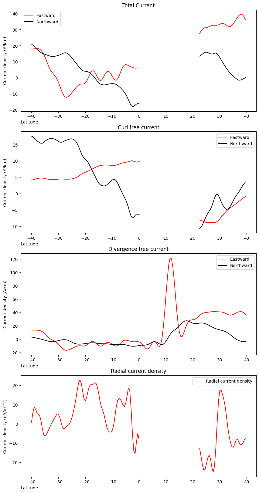
Simple line plots of the currents from the central latitudinal slice

The outputs in the datatree are enumerated, for each analyzed equatorial crossing included inside the timestamps. (“DSECS_output/0/currents”,”DSECS_output/1/currents” etc.)

print(data["DSECS_output/0/currents"].coords)
print(data["DSECS_output/0/currents"].data_vars)

Coordinates:
    Longitude  (x, y) float64 9kB 348.4 349.1 349.8 350.6 ... 350.5 351.2 351.9
    Latitude   (x, y) float64 9kB -39.96 -39.96 -39.96 ... 39.54 39.54 39.54
Data variables:
    JEastDf      (x, y) float64 9kB 12.75 12.97 13.34 ... 37.09 37.21 37.56
    JNorthDf     (x, y) float64 9kB 3.218 3.287 3.355 ... -2.858 -1.361 0.6997
    Jr           (x, y) float64 9kB 6.202 5.203 3.722 ... -0.896 0.6389 -0.2665
    JEastCf      (x, y) float64 9kB 4.798 4.568 4.314 ... -1.064 -1.587 -2.082
    JNorthCf     (x, y) float64 9kB 17.18 17.35 17.49 ... 3.934 4.322 4.705
    JEastTotal   (x, y) float64 9kB 17.55 17.54 17.66 ... 36.03 35.62 35.47
    JNorthTotal  (x, y) float64 9kB 20.4 20.63 20.84 20.96 ... 1.076 2.961 5.405

latitudes = data["DSECS_output/0/currents"]["Latitude"][:, 3]
fig, ax = plt.subplots(4, 1, figsize=(10, 20))
lineE = ax[0].plot(
    latitudes,
    data["DSECS_output/0/currents"]["JEastTotal"][:, 3],
    "r",
    label="Eastward",
)
lineN = ax[0].plot(
    latitudes,
    data["DSECS_output/0/currents"]["JNorthTotal"][:, 3],
    "k",
    label="Northward",
)
ax[0].set_title("Total Current")
ax[0].set_ylabel("Current density (A/km)")


lineE = ax[1].plot(
    latitudes, data["DSECS_output/0/currents"]["JEastCf"][:, 3], "r", label="Eastward"
)
lineN = ax[1].plot(
    latitudes, data["DSECS_output/0/currents"]["JNorthCf"][:, 3], "k", label="Northward"
)
ax[1].set_title("Curl free current")
ax[1].set_ylabel("Current density (A/km)")

# ax[0].set_title('Total Current (DF + CF)')

lineE = ax[2].plot(
    latitudes, data["DSECS_output/0/currents"]["JEastDf"][:, 3], "r", label="Eastward"
)
lineN = ax[2].plot(
    latitudes, data["DSECS_output/0/currents"]["JNorthDf"][:, 3], "k", label="Northward"
)
ax[2].set_title("Divergence free current")
ax[2].set_ylabel("Current density (A/km)")

liner = ax[3].plot(
    latitudes,
    data["DSECS_output/0/currents"]["Jr"][:, 3],
    "r",
    label="Radial current density",
)
ax[3].set_title("Radial current density")
ax[3].set_ylabel("Current density (nA/m^2)")

for axv in ax:
    axv.set_xlabel("Latitude", loc="left")
    axv.legend()

(Preview) Quicklook plots

from swarmpal.experimental import dsecs_plotting

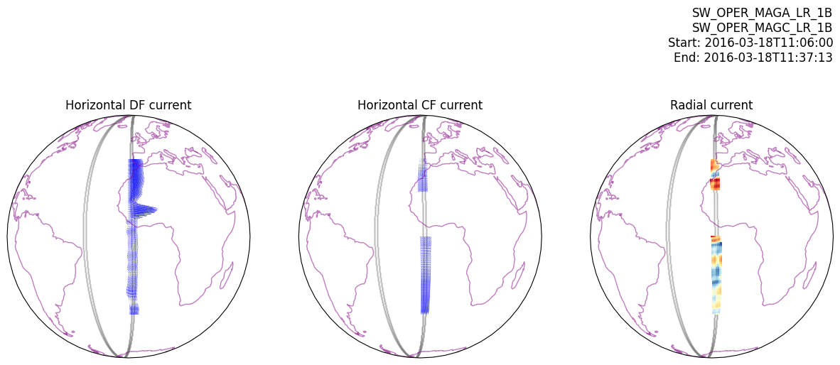
Plot a specific pass

dsecs_plotting.plot_analysed_pass(data, "DSECS_output", pass_no=0)

/home/docs/checkouts/readthedocs.org/user_builds/swarmpal/envs/main/lib/python3.11/site-packages/cartopy/io/__init__.py:242: DownloadWarning: Downloading: https://naturalearth.s3.amazonaws.com/110m_physical/ne_110m_coastline.zip
  warnings.warn(f'Downloading: {url}', DownloadWarning)

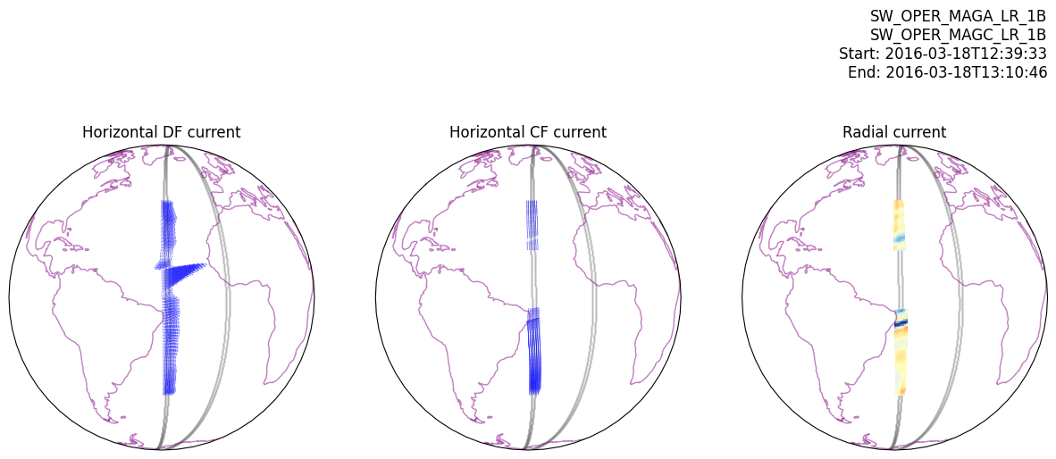
Automatically plot all passes

figs = dsecs_plotting.quicklook(data)

figs[0]

figs[1]

Create an animation of those quicklook plots (using ipwidgets)

(If you are viewing this on the web, it will not be interactive)

dsecs_plotting.quicklook_animated(data)

data.to_netcdf("dsecs_example.nc")